Fatigue Analysis, Damage calculation, Rainflow counting

Fatigue is the progressive and localized structural damage that occurs when a material is subjected to cyclic loading. Continued cycling of high-stress concentrations may eventually cause a crack which propagates and results in leakages. This failure mechanism is called fatigue.

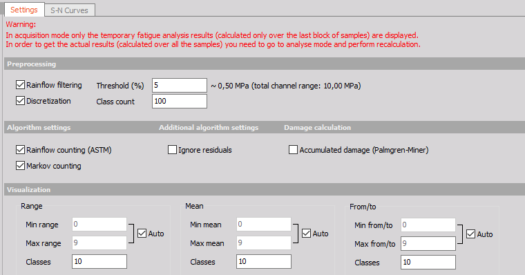
Before going into the fatigue analysis details, let us consider the following example. Say we wanted to break a metal rod that is not too thick. How would we tackle the task? In a brute-force way like the guy in the picture below or some other way? Well, if we asked a fatigue analysis expert he would probably suggest us to repeatedly bend both ends of the rod slightly upwards and downwards. And he would be right. The rod would break. Maybe not immediately, maybe not after one hundred repetitions, maybe not after one thousand repetitions, but eventually it would break.

Breaking a metal rod
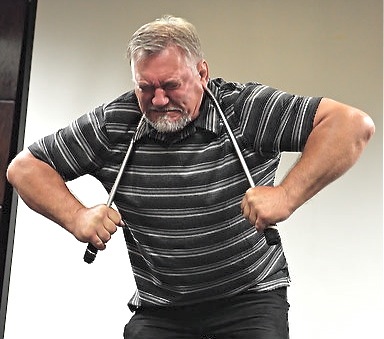
Image 1: Breaking a metal rod

 How to explain this phenomenon? Let us first describe the physics behind bending the rod. As depicted in the image below, bending induces the stress (σ) in the cross-section of the rod. Bending the rod upwards induces the positive stress, i.e., compression at the top and tension at the bottom of the cross-section (a), whereas bending the rod downwards causes the negative stress, i.e., tension at the top and compression at the bottom of the cross-section (b). When the rod is in the equilibrium position no stress is induced (c).

CompressionImage 2: Positive stress - compression at the bottom and tension at the top


TensionImage 3: Negative stress - tension at the bottom and compression at
the top


equilibrium positionImage 4: No stress-induced - equilibrium position


When bending is repeatedly applied for a sufficient period of time microscopic cracks are initiated in the cross-section of the rod. As the bending continues these tiny cracks are propagated until they grow to a point where the rod breaks. This phenomenon is called crack propagation.

As depicted in the figure below, cracks can propagate in three modes depending on the relative orientation of the load.

TensionShearTorsion
TensionImage 5: Tension


ShearImage 6: Shear


TorsionImage 7: Torsion


You probably don't care much about the broken rod from the example above, right? Well, what if the same rod was a part of a more complex and bigger structure, such as a bridge, an airplane or a train, and its fracture could cause a severe accident with people involved? Clearly, crack propagation poses serious problems of both design and analysis in many fields of engineering, especially in civil engineering where safety is of paramount importance. What makes crack propagation even more problematic is that is is very hard to explicitly detect and measure. Therefore, fatigue analysis engineers typically use implicit statistical and predictive tools described in the following chapters.

Demolished bridge
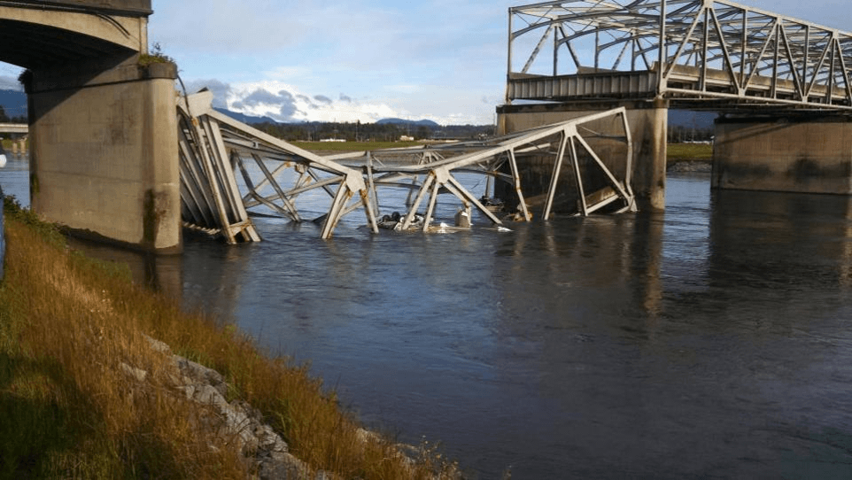
Image 8: Demolished bridge


In this chapter, we introduce some basic terms used in fatigue analysis and briefly describe the basics.

Load

Load is defined as any physical quantity that reflects the excitation or the behavior of a system or component over time. The most typical loads are:

  • forces,
  • torques,
  • stresses,
  • strains,
  • displacements,
  • velocities,
  • accelerations etc.

An example of a load signal is depicted in the figure below, showing vertical load measured on a truck transporting gravel. The changes in the mean originate from a loaded and unloaded truck, whereas the changes in the standard deviation are the result of different road qualities.


Example of a load signal in time domainImage 9: Example of a load signal


Cycle

A half-cycle is a pair of two consecutive extrema in the load signal, going from a minimum to a maximum or vice versa, as depicted in the image 10 below. A full-cycle is a cycle consisting of two consecutive half-cycles, as depicted in image 11 below.

Half cycleImage 10: Half-cycle


Full cycleImage 11: Full-cyle


The most important cycle characteristics are Range, Amplitude and Mean, defined as follows:

  • Amplitude = (Maximum - Minimum) / 2,
  • Range = Maximum - Minimum,
  • Mean = (Maximum + Minimum) / 2.

Cycle Counting Methods

Cycle counting methods are used to calculate the load spectrum of a load signal, i.e., number of cycles corresponding to each range in a load signal. An example of a load spectrum is depicted in the figure below. Typical cycle counting methods are rainflow counting and Markov counting described in the following chapters.


Cylce counting methodsImage 12: Cycle counting methods


Fatigue

Fatigue is the failure mechanism that is caused by repeated load cycles with amplitudes well below the ultimate static material strength. Formally, the fatigue process is divided into three stages:

  • crack initiation,
  • crack propagation,
  • unstable rupture and final fracture.

A repeated load applied to a particular object under observation will sooner or later initiate microscopic cracks in the material that will propagate over time and eventually lead to failure. Fatigue damage is typically cumulative and, therefore, unrecoverable.

Fatigue behaviour depends on many factors such as:

  • load type,
  • object size
  • stress/strain concentration and distribution,
  • mean stress/strain,
  • environmental effects,
  • metallurgical factors and material properties,
  • load rate and frequency effects.

Fatigue Life Prediction

Fatigue life prediction is the process of predicting fatigue life of a particular object under observation. According to ASTM fatigue life is defined as number of stress cycles that a specimen sustains before failure. Fatigue life prediction is of vital importance in order to assure product quality and safety.

Durability

Durability is the capacity of an item to survive its intended use for a suitable long period of time. Good durability leads to good quality, company profitability and customer satisfaction.


Explanation of SN curves

Generally speaking, S-N curves (also known as Wöhler curves) represent statistical models that characterize the material performance. S-N curve is defined as a graph of the cyclic stress against the logarithmic scale of cycles to failure. The figure below depicts two S-N curves, a red one and a blue one, corresponding to aluminum and steel, respectively. Let us take a closer look at the latter. If the cyclic stress of approximately 45 ksi* is applied to the steel the failure will occur after 104 cycles, whereas applying lower cyclic stress of approximately 40 ksi will result in failure after 105 cycles. Furthermore, at 30 ksi the S-N curve reaches the so-called endurance limit. The endurance limit is the amplitude of the cyclic stress that can be applied to the material without causing fatigue failure. Thus, if the cyclic stress of 30 ksi or less is applied to the steel failure will never occur. On the other hand, at 45 ksi the S-N curve reaches the so-called ultimate stress, defined as the maximum stress a material can withstand.


S-N curve for steel and aluminiumImage 13: Examples of SN curves for Steel and Aluminium, *ksi - kilopounds per square inch


S-N curves are derived from tests on material samples to be characterized (called coupons) where regular sinusoidal stress is applied by a testing machine which also counts the number of cycles to failure as depicted in figures (a), (b) and (c) below. This process is known as coupon testing. Each coupon test generates a point on the plot though in some cases there is a run-out where the time to failure exceeds that available test period. Analysis of fatigue data requires techniques from statistics, especially survival analysis and linear regression.

Image 14: Failure after 1 cycle


Image 15: Failure after 3 cycles


Image 16: Failure after 5 cycles


When designing the components engineers always try to keep the stress amplitudes below the endurance limit, way below the ultimate stress value. Since the material never fails below the endurance limit it is safe to be operated at such stress amplitudes.


The S-N curves model described in the previous chapter assumes that the material is subjected to a constant amplitude load, i.e., cycles to failure correspond to a constant cyclic stress amplitude, as depicted in the image 17 below. The next generalization is to consider a block load, i.e., consecutive blocks of constant amplitude load, as depicted in the image 18 below.

Image 17: Constant amplitude load


Image 18: Block load


In this case, the Palmgren-Miner damage accumulation hypothesis states that each cycle with amplitude Si uses a fraction 1 / Ni of the total life. Thus the total fatigue damage D is given by equation:

\( D =\sum_{i} \frac{n_{i}}{N_{i}} \)


where ni is the number of cycles with amplitude Si. Fatigue failure occurs when the damage D exceeds one.

Although Palmgren-Miner rule represents a useful approximation model in many circumstances, it has several major limitations:

  • It fails to recognize the probabilistic nature of fatigue.
  • In some circumstances, cycles of low stress followed by high stress cause more damage than the rule predicts. It does not consider the effect of an overload or high stress which may result in compressive residual stress that may retard crack growth. High stress followed by low stress may have less damage due to the presence of compressive residual stress.

Although fatigue analysis covers a very broad range of areas, such as mechanics, physics and statistics, we can simply define it as the process of analysing, modelling and predicting fatigue behavior. In order to summarize the fatigue analysis basics, let us consider the following example, illustrating a very simple fatigue analysis use-case in the car industry.

Suppose that a company, or some company division, is manufacturing drive shafts and a team of engineers is responsible for ensuring they meet performance, quality and safety requirements. Assuming that preliminary drive shaft tests were already performed and the team is now interested in the long-term analysis, what would be the next steps?

Typically, an engineering team would first gather as much statistical data as possible, such as target driver group (whether shafts will be used in family cars, trucks etc.), target driver behavior (average driving distance per year, average driving speed etc.), target driving conditions (road conditions, speed limits etc.) and so forth. Afterwards, statistical models describing the target environment would be derived. The models would, consequently, serve in a real-life testing, including real driving in the real environment, with all the required data acquisition taking place, such as measuring load applied to the driver shaft. Finally, the cycle counting methods would be applied to the measured load signals and statistical methods, such as S-N curves or Palmgren-Miner rule, would be used to check whether load amplitudes exceed the endurance limits of the steel, how often and how much they exceed it, whether the fatigue limit is exceeded, whether the Palmgren-Miner damage is exceeded etc. If the results did not comply with the recommended values, the shaft would probably have to undergo additional modifications and re-engineering.


Fatigue Analysis Module supports a wide range of fatigue analysis features and utils. Combined with Dewesoft X it represents a powerful all-in-one fatigue analysis solution allowing both acquisition and analysis of the fatigue data - everything in a single software package!

It is located under Strain, stress Fatigue analysis.

The module is organized into three main sections: Preprocessing, Counting methods (Algorithm settings) and Visualization. In fact, section organization follows a typical fatigue analysis workflow that starts with the input signal preprocessing, proceeds with the cycle counting and ends with the result visualization.

Image 20: Fatigue analysis module in Dewesoft


Remark:
In acquisition mode, only the temporary fatigue analysis results (calculated only over the last block of samples) are displayed. In order to get the actual results (calculated over all the samples), you need to go to analyse mode and perform a recalculation!

Each section represents a particular fatigue analysis stage and covers a subset of corresponding methods as follows:

  1. Preprocessing
    • Turning points filter
    • Rainflow filter
    • Discretization filter
  2. Counting methods
    • Rainflow counting (ASTM E 1049-85)
    • Markov counting
  3. Visualization
    • Range histograms
    • From/to matrices
    • Range/mean matrices
  4. Damage calculation
  • Accumulated damage (Palmgren-Miner rule)


The preprocessing section includes the turning points filter, rainflow filter and discretization filter.

Turning Points Filter

The Turning points filter detects local extrema, namely turning points, in the load signal. An example of turning point detection is depicted in the figure (a) below. The filter is applied to the input signal by default and cannot be disabled since the Fatigue Analysis Module requires a sequence of turning points as its input (instead of a full load signal).

Rainflow Filter

The Rainflow filter (also called the hysteresis filter) removes small oscillations from the signal, as depicted in the figure (b) below. All turning points that correspond to the cycles with the ranges below the given threshold are removed. The higher the threshold, the more turning points are filtered out, and vice versa. Rainflow filtering can significantly reduce the number of turning points, which can be of importance for both testing and numerical simulation. The Threshold parameter of value T corresponds to the T% of the absolute load signal range.

Discretization Filter

The discretization filter divides the range of a load signal into N equidistant bins and assigns each turning point to its closest bin. Figure (c) below depicts an example where signal ranging from -10 to 10 is discretized into 5 bins. Load signals are typically very stochastic (please refer to the first figure in the Fatigue Analysis Basics chapter), therefore, discretization is often applied to make them flatter and less stochastic. The number of bins is adjusted with the Class count parameter.

Both the rainflow filter and the discretization filter are activated in the Preprocessing section by ticking the appropriate checkbox, as depicted below.


Image 21: Preprocessing process in Dewesoft


Description of Markov counting method

Markov counting is one of the most straightforward cycle counting methods. It operates on consecutive pairs of turning points and calculates absolute ranges between them. The method is activated by ticking the Markov counting checkbox in the Algorithm settings section.


Image 22: Markov counting in Dewesoft

The figure below depicts an example of Markov counting in action. Clearly, the 6th turning point of the load signal is assigned a value of |5 - 2| = 3, i.e., the absolute difference between the 6th and the 5th turning point. Similarly, the 7th turning point is assigned a value of |4 - 5| = 1, i.e., the absolute difference between the 7th and the 6th turning point.


Image 23: Example of Markov counting algorithm


When large amplitude cycles (such as the cycle between the 5th and the 8th turning point in the figure above) contain smaller amplitude cycles, Markov counting fails to detect them. Since large amplitude cycles play an important role in fatigue life, this represents a major drawback of the method.


Rainflow counting is generally accepted as being the best cycle counting method up to date, and has become the industrial de facto standard. It is activated by ticking the Rainflow counting check box in the Algorithm settings section.

Image 24: Rainflow counting in Dewesoft


The idea behind the method is to detect hysteresis loops in the load signal, as depicted in the figure below. We'll refer to the hysteresis loops as the closed cycles. Parts of the signal that do not correspond to the closed cycles are the so-called open cycles or residuals. Simply said, closed cycles and residuals could be visualized as full-cycles and half-cycles, respectively.


Image 25: Rainflow counting - hysteresis loop


As opposed to the Markov counting, which fails to detect large amplitude cycles, the rainflow counting successfully detects them. As depicted in the figure below, it detects the large amplitude cycle (2,6) and the small-amplitude cycle (4,5) within.


Image 26: Rainflow cycle counting algorithm

Different rainflow counting standards, such as ASTM, DIN and AFNOR, differ with respect to the treatment of the residuals. In order to be as general as possible, the Fatigue Analysis Module supports both residual and non-residual mode. When Ignore residuals checkbox in the Additional algorithm settings section is checked, the residuals are omitted, otherwise, they are included in the results.


Image 27: Ignore residuals checkbox


In order to graphically represent the results the Fatigue Analysis Module uses the most common visualization techniques used in fatigue analysis: range histograms, from/to matrices and range/mean matrices. When an input channel corresponding to a load signal of interest is selected, the following new channels are mounted:

  • Preprocessing
    • Peak/valley channel
    • RF filter channel
    • Discretization channel
  • Rainflow counting
    • Range histogram channel (2-D)
    • Range/mean matrix channel (3-D)
    • From/to matrix channel (3-D)
  • Markov counting
    • Range histogram channel (2-D)
    • From/to matrix channel (3-D)

Remark:
The channels marked with 2-D and 3-D correspond to 2-D and 3-D graphs, respectively. The channels corresponding to the Preprocessing section represent intermediate fatigue analysis results and serve for information purposes only.

All the channels are depicted in the screenshot below.

Image 28: Channels from Fatigue analysis in Dewesoft


Range histogram is a 2-D graph representing the range distribution of a load signal. An example of a range histogram is depicted in the figure below. The X-axis and Y-axis of a range histogram correspond to the range and number of cycles, respectively. Thus, if a load signal contained 500 cycles of range 20 and 700 cycles of range 40, the entries of (X=20, Y=500) and (X=40, Y=700) would be added to the range histogram.

Image 29: Range histogram


A typical range histogram use-case would be to obtain the range histogram of a signal, rotate it over diagonal (swap the X-axis and Y-axis), overlay a corresponding S-N curve on top and check whether it stays well below the curve.

From/to matrix is a 3D graph representing the cycle distribution of a load signal. An example of a from/to matrix is depicted in the image below.

  • X-axis - From (cycle minimum)
  • Y-axis - To (cycle maximum)
  • Z-axis - Number of cycles

Image 30: From-to matrix displayed on the 3D graph


For example, the image below depicts a cycle ranging from 5 to 10. In this case From and To are assigned the values of 5 and 10, respectively. If a load signal contained 100 such cycles, entry of (X=5, Y=10, Z=100) would be added to the from/to matrix.

Image 31: Cycle ranging from 5 to 10


Range/mean matrix is a 3D graph representing the cycle distribution of a load signal. An example of a range/mean matrix is depicted in the figure below.

  • X-axis - cycle range
  • Y-axis - cycle mean 
  • Z-axis - number of cycles

For a detailed description of cycle range and cycle mean please refer to Fatigue Analysis Basics chapter

range-mean matrixImage 32: Range-mean matrix displayed on the 3D graph


For example, the figure below depicts a cycle ranging from 5 to 10. In this case range and mean are assigned the values of 5 = 10 - 5 and 7.5 = (10 + 5) / 2, respectively. If a load signal contained 300 such cycles, entry of (X=5, Y=7.5, Z=300) would be added to the range/mean matrix.


cycle from 5 to 10Image 33: Cycle ranging from 5 to 10


The visualization section is organized into three groups: Range, Mean and From/To, as depicted in the screenshot below. Each group controls the appearance of the corresponding graphs. For instance, Range group controls the appearance of the range histograms and the range/mean matrices. Min range and Max range parameters specify the minimum and maximum of the range axis, whereas the Classes parameter specifies the number of classes the range is divided into. 

When the Auto checkbox is ticked Dewesoft automatically calculates Min range and Max range from the input signal. Exactly the same concept goes for the Mean and From/To groups as well.


Visualization setup in DewesoftImage 34: Fatigue visualization setup in Dewesoft


Graph appearance can be additionally controlled in the Dewesoft settings window under Extensions > Fatigue analysis > Settings, as depicted in the screenshot below.


Show ticks setting in DewesoftImage 35: Settings for showing ticks at different positions


The Ticks parameter controls the position of the graph ticks. When Show ticks at class centers is selected the ticks are displayed exactly at the class centers, whereas Show ticks at lower-class bounds display them at the lower class bounds, as depicted in the figures (a) and (b) below, respectively.

Ticks at class centerImage 36: Ticks at class center


Ticks at lower class boundsImage 37: Ticks at lower-class bounds


Additional Fatigue Analysis Module settings are located in the Dewesoft settings window under Extensions > Fatigue analysis, as depicted in the screenshot below.


Use hard drive for calculationImage 38: Setting for using hard drive for calculation


Ticks

For the Ticks parameter please refer to the Visualization Settings chapter.

Use Hard Drive For Calculation

When analyzing extremely large data files with the Fatigue Analysis Module the operating system can run out of memory. In order to be as robust as possible and avoid such scenarios, the module supports a special Hard drive mode. In the hard drive mode all the intermediate data is stored on the hard drive instead of in the RAM, thus substantially decreasing the memory consumption. The hard drive mode is triggered by ticking the Use hard drive for the calculation check box. The mode, however, significantly reduces the performance and results in higher processing times. Therefore, it should be used only in cases where out-of-memory problems occur.


In this chapter, we demonstrate an example of a complete fatigue analysis workflow using the Fatigue Analysis Module and Dewesoft. Let us start with a simple signal, named Stress data, depicted in the screenshot below. The signal is stochastic and has several turning points.


Stochastic signal exampleImage 39: Stochastic signal example


First, we activate the Fatigue Analysis Module located under Strain, stress Fatigue analysis. After activating the module the setup screen appears, as depicted in the image below. We assign an input channel to the module by ticking the Data checkbox on the left-hand side of the screen. We won't be using any preprocessing, therefore, the Rainflow filtering and Discretization checkboxes are all left unchecked. In order to apply both counting methods, we tick the Rainflow counting and Markov counting checkboxes.

The next part is the visualization. After ticking all three Auto check boxes Dewesoft automatically assigns the values of 0 and 9 to Min and Max edit boxes. Clearly, since 0 and 9 represent the minimum and maximum of the input signal. For clearer visualization, the Classes parameter is set to 10. Thus, each class has width of 1 = (9 - 0 + 1) / 10. Dividing the range into 11 classes, for instance, would not result in the whole number, since (9 - 0 + 1) / 11 = 0.91!

Settings for analysis example in Fatigue moduleImage 40: Settings for analysis example in Fatigue module


Finally, we navigate to the Review tab and click the Recalculate button. After recalculation, the result screen is displayed, as depicted in the image below. The screen contains five graphs, i.e., the range histogram and from/to matrix corresponding to the Markov counting, and the range histogram, from/to matrix and range/mean matrix corresponding to the rainflow counting.


Example of Fatigue analysis screen in DewesoftImage 41: Example of Fatigue analysis screen in Dewesoft


The results obtained in the previous chapter can be optionally exported to a broad range of file formats. Let us, for example, export the data to a text file format. We navigate to the Export tab, as depicted in the screenshot below, and choose the Text/CSV (*.text, *.csv) from the list of supported file types. After selecting the appropriate channels on the right side of the screen, we click the Export button.


Export data sectionImage 47: Export data from Dewesoft


When the export has finished the exported text file appears in the Existing files list box. Double-clicking the file opens it in an external text viewer (such as Notepad), as depicted in the screenshot below.

Remark:
When a full-cycle is detected by rainflow counting it contributes a value of 1 to the total number of cycles, whereas a residual contributes a value of 0.5. Therefore, range histograms and range/mean matrices often contain values such as 0.5, 1.5, 2.5 etc. If we ticked the Ignore residuals check box the residuals would be ignored and 0.5 values would disappear from the results below.


UNV export fileImage 48: Example of the exported TXT file


Perform damage calculation according to the Palmgren-Miner rule

According to Miner's Rule, when damage is equal to 1, failure occurs. The definition of failure for a physical part varies. It could mean that a crack has initiated on the surface of the part. It could also mean that a crack has gone completely through the part, separating it.

In order to make a damage calculation, you need to add an S-N curve in the S-N curve editor.

Image 42: S-N curve editor


Please make sure that the input units of the signal match the units of the S-N curve. In the S-N curve editor, you can add your own S-N curve, define the name, unit, axis type, and the number of points. When you are done with defining the curve, click the Save button.


Image 43: Adding new S-N curve


 When the S-N curve is added, go back to the Fatigue analysis module and select option Accumulated damage. When you select this option, you will be able to go into the S-N curves tab.

Accumulated damageImage 44: Accumulated damage option in Dewesoft and S-N curves tab

The next step is to go to the S-N curves tab and select the correct S-N curve.


Image 45: SN curves selection

Only the overall damage in the defined area of the S-N curve will be calculated. If your stress level or a number of cycles is outside of the predefined area, the damage will not be added to the overall damage.


S-N curve limitsImage 46: Defined level of damage calculation in S-N curve area

 As seen from the image above for this specific S-N curve, only the damage calculated from the stress levels and cycle numbers inside the orange area will be added to the overall damage calculation.