Order Tracking Measurement and Analysis

Order tracking method is used to extract the harmonic components related to the rotational frequency of the machine. Order tracking is used in the analysis of vibration signals from rotating machines. There we use order spectrum instead of the frequency spectrum. An order spectrum gives the amplitude and the phase of the signal as a function of the harmonic order of the rotation frequency.

Analysis of vibration signals from rotating machines is often preferred in terms of order spectrum rather than the frequency spectrum. An order spectrum gives the amplitude and the phase of the signal as a function of harmonic order of the rotation frequency. This means that a harmonic or subharmonic order component remains in the same analysis line independent of the speed of the machine. The technique is called tracking as the rotation frequency is being tracked and used for analysis.

The order tracking method is used to extract the harmonic components related to the rotational frequency of the machine. The machine vibration pattern is a mixture of excitation frequencies, usually related to rotational speed (such as unbalance, eccentricity, bearing faults and others) and machine response function, which relates to machine natural frequencies based on the structure and mounting of that machine.

With order extraction, we can see a specific harmonic component which relates to a certain machine fault. That is - the first order (harmonic) usually relates to unbalance of the machine, the second harmonic often relates to eccentricity, such as if we have for example 9 rotor blades, the 9th harmonic relates to errors on the blades. Or, if we have for example 31 teeth on a gear, then the 31st harmonic will show the gear mesh frequency.

These are excitations, forces which produce vibration accelerations. The ratio between excitation and system response is defined by the system transfer curve. The final measured vibration of the system is a product of the excitation force and the system transfer curve. Since the transfer curve is fixed, we get different responses for excitations at different rotation speeds. When the excitation passes natural frequency, we get the so-called resonance with increased vibration amplitudes, which could be fatal to the machine.


Order tracking 3D displayImage 1: Example of Order tracking 3D display


This page should give you a rough idea what 1st, 2nd, ... order means and what might be their possible source.

1st order = imbalance

The first order is the shaft frequency, so if the first order is the main reason for high vibration, this is related to an unbalanced shaft or blade.


1st orderImage 2: Explanation of 1st order


Imagine a blade or shaft or any rotating part that has a higher weight at one side. This weight will rotate with exactly the rotational speed (1st order), create a force and, therefore, a vibration frequency which is exactly the rotation speed or first order. So high amplitudes of first orders indicate an unbalanced system.

1st and 2nd order = misalignment


1st & 2nd orderImage 3: Explanation of 1st & 2nd order


If a high second order is observed in the vibration spectrum of a machine, it often indicates a misalignment of two coupled engines. So, two times per revolution (2nd order) the shaft is bent and causes a vibration force, which is transmitted to the mechanical structure and creates a vibration.

Diesel and gasoline engines

In a diesel and gasoline engines, we can observe that 2nd, 3rd or 6th order are almost all the time dominant, why?

  • It depends on the cylinder count of the engine. Let's assume we have a 4 cylinder 4 stroke engine. One cylinder is fired every 2 revolutions, so we would get 0.5 order vibration if we would have a 1 cylinder engine.
Order tracking other ordersImage 4: Explanation of other orders
  • With a 4 cylinder engine the firing of the 4 cylinders is distributed over 4 revolutions, 2 rev/4 = 0,5 rev so one of the 4 cylinders will fire every 0,5 revolutions. This will lead to high second order vibration.
  • A 6 cylinder 4 stroke engine will produce high 2 rev/6 = 0.33rev → 3rd order.


Rotating machines produce repetitive vibrations and acoustic signals related to the rotational speed. These relationships are not always obvious with standard dynamic signal analysis, particularly with variations in the rotational speed. A measurement technique called order analysis is the secret to sorting out all the many signal components that a rotating machine can generate.

Order tracking is a family of signal processing tools aimed at transforming a measured signal from the time domain to angular (or order) domain. These techniques are applied to asynchronously sampled signals (i.e. with a constant sample rate in Hertz) to obtain the same signal sampled at constant angular increments of a reference shaft. In some cases, the outcome of the order tracking is directly the Fourier transform of such angular domain signal, whose frequency counterpart is defined as "order". Each order represents a fraction of the angular velocity of the reference shaft.

Order tracking is based on a velocity measurement, generally obtained by means of a tachometer or encoder, needed to estimate the instantaneous velocity and/or the angular position of the shaft.

Rotating machines under operational conditions require additional analysis such as order tracking. Compared to normal FFT, order spectra are based on orders (periods per revolution) instead of frequency (periods per time). With this method, you can separate the frequency components which are related to engine speed and those that are related to the structure.


3D graph of Orders regarding different Speed'sImage 5: 3D graph of Orders regarding different Speed's


Dewesoft X software provides a powerful and very easy-to-use order tracking module for fast and efficient results. The data and the RPM information is recorded simultaneously in the time domain and re-sampled in the order tracking module. Therefore, we can show a narrow band FFT, waterfall spectrum, and still keep all other convenient functions in the time domain.

The classical problem of smearing of the frequency components caused by speed variations of the machine is solved by using order analysis. In situations where the frequency components from a normal frequency analysis are smeared together, proper diagnosis is order analysis.

Of particular interest is the analysis of the vibrations during a run-up or a coast-down of a machine in which case the structural resonances are excited by the fundamental or the harmonics of the rotational frequencies of the mechanical system. Determination of the critical speeds, where the normal modes of the rotating shaft are excited, is very important on large machines such as turbines and generators.

Use of an FFT analyser in the normal sampling mode with a fixed sampling frequency (non-tracking) and plotting of the spectrum at certain fixed steps in the rotation speed of the machine gives the Campbell diagram (3D waterfall type of a plot, where vibration levels as a function of frequency are plotted against rotation speed (RPM) of the machine (plotted vertically). This means that the harmonic components appear on radial lines through the point (0 Hz, 0 RPM) while structural resonances appear on vertical straight lines (constant frequency lines). The smearing of the components, which appears because the time window used for the individual spectra represents a certain sweep in the speed, is, however, a disadvantage. The power of the components becomes spread over several lines. In particular, high-frequency components in the spectrum, such as tooth mesh frequencies, might be smeared so much that details in sideband structures are lost in the analysis. This is the main reason why order analysis is used instead.


Comparison of Frequency waterfall vs. Speed and Order waterfall vs. SpeedImage 6: Flat projection comparison of Frequency waterfall vs. Speed and Order waterfall vs. Speed


3D comparison of Frequency waterfall vs. Speed and Order waterfall vs. SpeedImage 7: 3D projection comparison of Frequency waterfall vs. Speed and Order waterfall vs. Speed


For order tracking, the time record is measured in revolutions and the corresponding FFT spectrum is measured in orders. Just like the resolution, delta f [Hz], of the frequency spectrum, equals 1/T, where T [s] is seconds per FFT-record, the resolution of the tracked analysis, delta ord [ORD], equals 1/rev, where rev [REV] is revolutions per FFT-record. For the analysis with one or more revolutions per record, the resolution of the spectrum is equal to or better than 1 ORD. The result of the analysis is a high-resolution order-spectrum, where the individual orders or fractions of orders, relate directly to the various rotating parts of the machinery.

Tracking analysis (with use of an FFT analyser) is an analysis by which the harmonic pattern of the vibration signal from a rotating machine is stabilized in certain lines independent of speed variations. This means that all the power of a certain harmonic is concentrated in one line and the smearing that would result in normal analysis is avoided.


Before we start explaining all the different options of the setup, let's check at first why we need the order tracking module.

An electrical scooter motor standing on a rubber foam is analysed. The RPM is controlled by DC voltage and measured by an optical probe (reflective sticker on a shaft) and the vibration by an acceleration sensor mounted on top.


Electric motor equipped with acceleration sensor and tachoImage 8: Electric motor equipped with acceleration sensor and tacho


FFT spectrum at 800 rpm

In the first example, the engine is running at a constant speed of 800 rpm.


FFT spectrum at a constant 800 RPMImage 9: FFT spectrum at a constant 800 RPM 


When we look at the vibration spectrum, the lowest frequency of the highest peak is 13,73 Hz (13,73 * 60 = 823 rpm), which is most likely the first order. The next peak could be the 16th order (13,73 * 16 = 219,7 Hz).

When we increase the RPM now, the distance between some of the spectral lines gets bigger. We call the lines moving with RPM harmonics. They can be calculated by multiplying the base frequency with an integer number.

FFT spectrum at 1950 rpm

Then we run the engine at a constant speed of 1950 rpm.


FFT spectrum at a constant 1950 RPMImage 10: FFT spectrum at a constant 1950 RPM


The first order is again the lowest frequency peak at 32,04 Hz (32,04 Hz * 60 = 1922 rpm). Around 518 Hz, is most probably the 16th order. The 1754 Hz more or less stays the same and doesn't seem to be related to rpm (compare with 800 rpm measurement).

So, the spectrum consists of harmonics of the rotation speed and other frequencies.


Of course, it would take too much time to make an FFT for each RPM, so we can try to use the FFT during engine runup or coast down. The following experiment shows the FFT while the engine is slowing down from 1700 to about 1400 rpm.


FFT of an engine while in coast-down from 1700 RPM to 1400 RPMImage 11: FFT of an engine while in coast-down from 1700 RPM to 1400 RPM


When you compare the spectrum with the ones before, you see that there are no sharp lines anymore. The reason is that the rpm is changing while the FFT still needs time for calculation. This effect is called smearing.

Furthermore, from its nature, the FFT always has a frequency and an amplitude error.

To demonstrate, we generate a simple 100 Hz sine wave using the Dewesoft X mathematics (sine(100)). When we use a sampling frequency of 2048 Hz and an FFT with 1024 points we get (because of Nyquist criteria) a line resolution of exactly 1 Hz. Amplitude and frequency in the FFT are correct. Now we change the sine wave to 99.5 Hz. The energy of the peak is now distributed to both neighbor lines at 99 and 100 Hz, therefore, the amplitude is also not exact anymore.


Example of FFT SmearingImage 12: Example of FFT Smearing


In real life, it is very unlikely that the input signal will be at a constant frequency directly at the FFT line. Different windowing algorithms are designed for each application (flat top for example shows the correct amplitude).

In Dewesoft X, the FFT calculation time window is shown as a yellow frame in the overview instrument in Analyse mode if you click on the FFT.


Calculation time window adjustmentImage 13: Calculation time window adjustment


Manual order tracking would mean setting up each constant rpm sequentially, e.g. 600, 700, 800 then manually extracting the peaks from the FFT, and sorting them out to find the orders. You cannot be absolutely sure you will catch the right peaks (some frequency lines are not related to rpm and you can mix them up).

Using FFT during run-up/coast-down would result in unprecise measurement because of smearing and other FFT disadvantages.

With the Order tracking module of Dewesoft X, the order analysis is very easy to set up and easy to use.

The Dewesoft X order tracking module is used for e.g. vibration analysis on engines or other rotating machinery, both in development and optimization. With the small, handy form factor of the Dewesoft instruments (DEWE-43, SIRIUSi), it is also a smart portable solution for service engineers coping with failure detection.

The order tracking module is included in the DSA package (along with other modules like torsional vibration, frequency response function, ...).

How does it work? - Usually a run up or coast down of the engine is done. The measured vibration sensor data is calculated according to the angle sensor data, split up into orders, which can then be analysed across the whole rpm range. With order tracking the frequencies can be separated into those related to the RPM and spurious ones. The powerful visualisation and mathematic options lead to a clear picture of the situation.

Furthermore, calculations can also be done offline (after the measurement), like with most of the other modules, e.g. if a very high sampling rate is required or the CPU of the used computer simply is too weak.

If the powerful integrated post-processing features of Dewesoft X are not enough, you can even export the data to several different file formats.

System overview

Depending on what to analyze, e.g. acceleration sensors, microphones or pressure sensors are used to the analog input to measure sound/vibration. If they are e.g. voltage or ICP type, they are connected to the SIRIUS ACC amplifier or DEWE-43 with MSI-ACC adapter.

For the angle sensor, you have various possibilities: you can use either an Encoder with individual pulse count, CDM- 360/-720 or a simple tacho probe with 1 pulse/revolution (TTL or analog output) or 60-2, 36-2 tooth wheel sensor. If the RPM is changing slowly and the phase information is not of interest, the RPM can also be derived from any kind of signal (e.g. 0...20mA, which equals 0...6000rpm) or data channel, e.g. the CAN bus of a car.


Different signal acquisition optionsImage 14: Different signal acquisition options


To add Order tracking module in Dewesoft X  go into Measure mode, Channel setup and click on More... Search for Order tracking and select it.

Order tracking iconImage 15: Order tracking icon


The input mask of the order tracking module is split into the following sections:

Inputchannels: switch the output channels with arrow buttons and see preview values
Output
channels: switch the output channels with arrow buttons and see preview values
Frequency channel setup
defines the type of angle sensor (e.g. Enc-512, Tacho, Geartooth)
Reference signal - binningsets the RPM limits, the bin axis range, delta bin width, direction runup/coastdown/both/first, and supports a user-defined reference channel used as the bin axis.
Order FFT setup
specify maximum orders and the resolution (e.g. 1/16th order), order FFT vs. time, order FFT vs. RPM and order domain harmonics
Time FFT setup
defines the change calculation method from resampled data to FFT, time-domain harmonics and update rate on RPM change
Common properties
define the harmonic list, FFT window, data collection and bin update modes, scaling and spectral weighting.


In most of the cases, the analysis will be done with a vibration sensor. Just enable the desired channel(s) in the list on the left upper side of the module setup. Basically, any analog input can be used, here are some examples:

  • acceleration sensor
  • microphone
  • pressure sensor
  • output of the rotational vibration / torsional vibration module

Frequency channel setup

For determining the engine speed (rpm), an RPM sensor is needed. A lot of different sensors are supported.

In the Frequency source drop-down menu, you can choose between Counters, Analog pulses or RPM channel. Sensor menu will let you select the sensor you have created and saved in Counter sensor editor.  From the Frequency channel, you select the channel that is connected to your sensor.

You can access the Counter sensor editor in Options / Editors / Counter sensors or by pressing the "..." button.

Acceptable sensors for order tracking are for example

  • Digital
    • Tacho probe (1 pulse/revolution; connect to analog or digital input)
    • Encoder (e.g. 1800 pulses/revolution or CDM-360 / CDM-720 or 60-2; connect to Counter input)
  • Analogue
    • Geartooth sensors (36-2 or 60-2 sensor connect to an analog input)
  • any RPM channel 
    • Math channel, analogue voltage or RPM from CAN bus; but when using an RPM channel the phase of the harmonics cannot be extracted relative to the rotational angle, because there is no zero-angle information. Instead the phase can be determined relative to the 1st order absolute phase.

Counters

Select Counters if you connect an Encoder to the Dewesoft instrument Counter input (usually 7pin Lemo connector).

An encoder (e.g. 1800 pulses/revolution) or CDM (CDM-360, CDM-720) or Tacho (digital = TTL levels) or tooth wheel sensor (60-2) can be used. The counter setup in the background is then controlled (locked) by the Order tracking module, the counters will not be accessible (greyed out), to prevent double-usage.

In Counter mode, you can optionally set the filter, to suppress glitches/spikes shorter than the shown value (100ns...5μs). The optimal setting is derived from the following equation:

The biggest error is caused by improper mounting of an encoder. There are different mounting errors using a coupling, such as parallel, skewed, angled. The error will appear as periodic angle/frequency deviation during constant engine speed.

The easiest way is using a tacho probe with digital output. It can be directly connected to the Dewesoft instrument's counter input and is easy to mount. For example, the optical tacho probe only requires a reflective sticker on the rotating part, see Image 8.

Analog pulses

If you have a tacho probe (1 pulse/rev, optic, magnetic or any other type) with analog output signal, you can just connect it to an analog input (e.g. SIRIUS-ACC module) and use the analog setting of the frequency section.

Here example signals of a magnetic and an optic probe are shown.

Optic probe signalImage 16: Optic probe signal


Magnetic probe signalImage 17: Magnetic probe signal


Beyond that, also 60-2 and 36-2 analog signals from the crank sensor (inside nearly every vehicle) are supported.

Click the ... button to adjust the correct trigger level. You can also use the Find algorithm button, which will automatically determine the best possible value. Please take care when using a magnetic probe, that also the induced voltage will change depending on the RPM, resulting in a different trigger level. Therefore perform some test runs across the interesting RPM range to find the best trigger level.

Below, an example of 60-2 analogue sensor is shown.

Angle sensor math setupImage 18: Angle sensor math setup

60-2 analogue sensor signalImage 19: 60-2 analogue sensor signal


HINT: If machines with highly dynamic rpm, or with a high rotational vibration are analyzed (big rpm deviations during one revolution), and also high orders should be extracted, an encoder or a tacho probe with more than one pulse/rev. (180p/rev or higher) is recommended, to get higher accuracy.

Reason: The order tracking algorithm resamples the time domain data into the angle domain. If we get more information from the RPM probe, we have more pulses per revolution and the resampling to the angle domain will be much more accurate!


RPM channel

You can also use any signal or channel as input, which directly represents the RPM (e.g. 0...10V equals 0...5000 rpm).

The disadvantage, however, is, that there is no zero-angle information, and therefore extraction of the phase angles of the single orders is not possible.

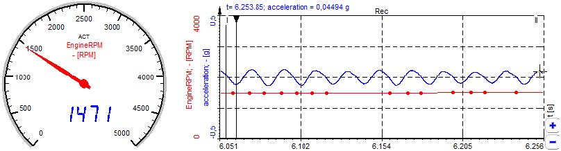
Following example shows an RPM signal from CAN bus inside a vehicle (red line). Note that the sampling points are asynchronous. The blue line is the output signal of an acceleration sensor.

CAN bus RPM signalImage 20: CAN bus RPM signal

Speed ratio

Speed ratio settings, found under Frequency channel setup.

With speed ratio settings it is possible to account for gearing ratios between a rotation source and the rotation at another component, where the frequency channel sensor might be located. For example, for practical reasons it might be necessary to perform the frequency channel measurement on a machine component different from the main crankshaft. By using the speed ratio settings the frequency channel can be converted to represent the speed of another component like e.g. the crankshaft. 

If the measured frequency channel is measured on an output shaft of a system and the order tracking should relate to the input shaft of that system, then the speed ratio should be set to input/output.
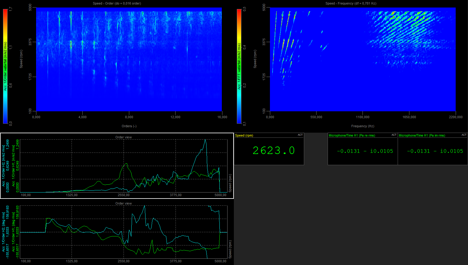
The reference channel are used as an additional axis or dimension, tagged to related order results. For example, a reference channel can be measured RPM, or temperature for which order results are found at each bin - creating 3D waterfall spectrograms, and extracted harmonics vs reference.

To cover all vibration characteristics, a run-up or a coast-down of the engine has to be performed.

Image 21 represents a recording of RPM over time. All terms that you will encounter during the setup of Order Tracking are visually presented. In this illustrated example the Reference channel is set to RPM, but it could also have been set to another measured channel (having another physical quantity than RPM).

Representation of Order tracking terminologyImage 21: Representation of Order tracking terminology, when using an RPM reference channel.

Reference signal - binning

Select the Upper- and Lower limit to specify the Reference Channel range used for calculation, and whether you want to calculate the waterfall spectrum and order extractions while doing a run-up, coast-down, both or based on the First Direction.

Image 22: Reference signal - binning, parameter section.
In the picture the reference channel is set to a channel measuring temperature. The bin settings will related to that REF channel. 


Upper- and Lower RPM relate to the Frequency channel and is used in order tracking to correctly perform the dynamic resampling from the time domain to the angle domain. 


Delta defines the bin width of the REF axis in waterfall spectra and in extracted order domain harmonics.

Hysteresis is used to determine when measured data is assigned to another bin. Hysteresis is described in percentage of the Delta bin width. Assigning data to another bin will only be considered if the reference value crosses the bin edge by more than the hysteresis percentage.  

Common properties

Image 23: Common properties setup

To extract the orders simply enter the wanted number in the Harmonics list field. Separate multiple entries with the semicolon (;). In the example above the 0.5 sub order, and the 1st, 2nd, 3rd, 36th order are selected. If the extracted order falls between discrete order resolution steps, the closest fitting resolution will be taken, so if the resolution is 1st order and 1.8 is extracted, 2nd order will be used.

FFT window & Amplitude define the used time weighting function and the amplitude scaling of your measured spectral data. You can learn more about FFT windowing in the FFT course.

Data collection can be done in two ways:

On center of bincollects data closest to the center of the bins only
Continuouscollects data through the entire bins


Image 24: On center of bin collection presentation

Bin update determines how the collected data will be processed. It defines if all the results relating to the reference channel (vs. reference results) should be updated:

Alwaysif you have more run-ups or coast-downs, only the newest spectral bin values will be used in the output array.
First timeif you have more run-ups or coast-downs, only the first run spectral bin values will be used in the output array.
Averageif you have more run-ups or coast-downs, the element of the output array will be calculated as an average between old and new spectral bin values for each individual bin.
Maximumif you have more run-ups or coast-downs, the elements of the output array will contain the maximum spectral bin values for each individual bin.

The output results affected by the Bin update setting is:

  • Order domain harmonics
  • Order waterfall vs. reference
  • FFT waterfall vs. reference
  • Overall RMS vs. reference

Image 25: Bin Update settings and the dependent output channels

Spectral weighting is supported in the order analysis module with the following functions: 

Spectral weighting types supported directly in the Order analysis module.


  • Acoustic weighting - A- and C-weighting are used for sound pressure signals. When analyzing sound and noise signals acoustic weighting filters can be applied in order to take audible human perception into consideration.

  • Integration/Differentiation - Integration/Differentiation functions are used mainly for vibration signals to change the physical quantity. A typical scenario for this is when transforming data from the acceleration domain to the displacement domain. The table below illustrates how integration and differentiation functions can be used to transform vibration related physical quantities:

Domain transformations for vibration quantities when using integration and differentiation.

Skip missing bins


Empty bins typically appear when the Delta bin width is too narrow to capture the number of cyclic revolutions required to produce a spectrum. The required number of revolutions for each spectrum is the reciprocal of the Order resolution - better resolution require angle data from more revolutions.

  • If ‘Skip missing bins’ is enabled, all REF bins that miss revolutions for producing a spectrum will stay empty.

  • If ‘Skip missing bins’ is disabled, all REF bins that miss revolutions for producing a spectrum will use an overlapping amount of revolutions from previous REF bins that match the missing part required for producing a spectrum.

Order FFT setup properties

 In the Order FFT setup, you can enable or disable different options to tailor the acquisition to your needs.

Order domain harmonics
enable or disable harmonic channels, that are created from your entry in Harmonic list under Common properties, and are displayed in 2D Graph
Order waterfall vs. referencecreate channels that are used by 3D graph for the display of Orders in relation to the RPM or another selected Reference Channel. 
Order resolutiondefine the number of lines between two orders 
Maximum ordersets the maximum displayed order (To set the Maximum order to analyse go to Options / Settings / Extensions / Order tracking)
Phase referencesets the phase information relative to the keyphasor position of the angle sensor, or relative to the absolute phase of the 1st order.
Order waterfall vs. timecreate an order waterfall that is updating in regards to Time FFT setup's Update on time field 
Overlapused to increase the rate of Order waterfall vs. time calculations by setting an FFT sample block overlap percentage
Depending on the Upper RPM and the Maximum order used, the OT module will output a warning if the used sample rate is too low.

For example, set Upper RPM at 6000 and Maximum order at 64. The minimum required sample rate is calculated like this:

First-order at max speed: 6000 rpm / 60 = 100 Hz; so the highest order will be 100Hz * 64 = 6400 Hz. Because of order FFT analysis, the sampling frequency must be doubled to fulfil the Nyquist criteria: 2 * 6400 = 12800 Hz.

In an FFT, if the line resolution is 0.5 Hz, the required data window must be 2s. The same is true for the ordered resolution: If the resolution is set to 0,25 orders, 4 revolutions are required for one data block.

The higher the required order resolution, the more slowly the rpm must change.

Order domain harmonics


Order domain harmonics are complex channels displayed on the 2D graph. In the Harmonic list section, you define which harmonics you want to extract.

Extracted Order domain harmonicsImage 26: Extracted Order domain harmonics


Order waterfall vs. reference

Order waterfall vs. reference monitors current values of orders. You define the order resolution and the maximum order that will be shown on a 3D graph.


Order waterfall vs. RPMImage 27: Order waterfall vs. reference


Order waterfall vs. time

Order waterfall vs. time monitors orders through time and not only the current values. The channel is updated for every new order FFT being calculated.

Order waterfall vs. timeImage 28: Order waterfall vs. time


This will extract specific orders from the order waterfall plot to be used as channels, so it is possible to draw a specific order over time, or over engine speed.

To extract the orders simply enter the wanted number in the Harmonics list field. Separate multiple entries with the semicolon ";". For example, if you wish to extract 1st, 2nd and 3rd, 4th and 5th order, simply input 1;2;3;4;5 and press Enter. If the extracted order falls between discrete order resolution steps, the closest fitting resolution will be taken.

Time domain and order domain harmonics are both complex channels. To get the amplitude from the complex number, use the ABS function in the Math module.

abs('AI 1/Order H1')

To get the phase angles from complex numbers use the ANGLE function in the math module.

angle('AI 1/Order H1')

To get the real and imaginary part as separate channels out of the complex number, use two math formulas:

Real = real('acc/Time domain'[0])
Imaginary = imag('acc/Time domain'[0])

In the example above, the index [0] will show 1st harmonic, index [1] will show 2nd, and [2] the 3rd harmonic.

Extracting interharmonics

In order tracking module there is an option to extract fractional order components or interharmonics. Enter the number in the harmonic list section. Use "." as decimal separator. For example, 0.5 ; 1.2 ; 3.87 ; etc..

Order domain harmonics and interharmonics are complex channels displayed on the 2D graph.

Extracted 0,5th HarmonicImage 29: Extracted 0,5th Harmonic

Time FFT setup properties

In this section, you define the frequency domain spectral properties, and properties for harmonic extraction in the time domain.

In the Time FFT setup section the following data results can be selected as output channels:

  • Time domain harmonics - Complex output values with magnitude and phase information of the defined harmonics over a time axis. In the Harmonics list you define the harmonics that you want to extract.

  • FFT waterfall vs. reference - Frequency spectra over the defined range for the Reference Channel.

  • Overall RMS vs. reference - Overall RMS values over the defined range for the Reference Channel.


The FFT resolution and data block length is per default automatically set from the sampling rate, Order resolution and Maximum order.

Time-domain harmonics

This is a complex output channel showing the amplitude of harmonics in a time domain. In the harmonics list section, you define the harmonics that you want to extract.

Amplitudes of harmonics in time domainImage 30: Amplitudes of harmonics in time domain

The parameters Update on reference change (Delta) and Update on  parameters are used to define when new harmonic values are extracted on the time axis.

Update settings for Time domain harmonics 


FFT waterfall vs. reference

If FFT waterfall vs. reference is enabled, the Time FFT waterfall spectrogram will have a defined number of lines for every REF bin. The resolution is calculated from the Maximum order, sample rate and order FFT block size. For better understanding, the delta frequency is also shown. 

By default, the resolution is set to Auto. You can manually change the FFT resolution in the FFT waterfall diagram by selecting a value from the FFT lines drop-down menu.

Example of difference in calculated and displayed data:

Difference between left: Df = 24 Hz; right: Df = 6 HzImage 31: Difference between left: Df = 24 Hz; right: Df = 6 Hz

The second picture shows much sharper lines and separates much clearer into single frequencies.

Overall RMS vs. RPM

RMS calculation depends on FFT waterfall resolution

This channel shows the overall RMS amplitude over the defined reference channel range.

RMS of signal over different RPMImage 32: Overall RMS of a signal over a defined RPM range


Order domain harmonics are extracted in "orders over reference bin values", shown on a 2D graph.

Marked 1st, 16th and 32nd harmonicImage 33: Marked 1st, 16th and 32nd harmonic

The graph above shows a vibration spectrum of an electrical scooter motor, standing on rubber foam. The three major orders are marked (1st, 16th and 32th). It is also possible to extract them and see the amplitudes and phases over rpm.

This is the old way but still applies, especially if you want to monitor the behavior of extracted orders over the whole time interval (Order domain harmonic values get updated, when we hit reference values that was already used).

Please use the XY recorder for displaying the extracted data:

XY recorder IconImage 34: XY recorder Icon

First, pick the OT_Frequency channel from the channel list (x-axis) on the right side, then assign the abs('signal/Time domain'[0]) channel (y-axis).

Amplitudes and phases of harmonicsImage 35: Amplitudes and phases of harmonics


As the order tracking is done during a run up or coast down, the visualisation instruments show the vibration spectrum (and the orders) over RPM or another selected reference channel, and frequency. Single order lines can additionally be extracted.

Automatic display mode

With the order tracking module enabled when you start the measurement, Dewesoft X will automatically generate a predefined display setup showing the major signals for a quick start.

In the picture below, the automatic display configuration is shown. The visual controls in the bottom left of the screen are 2D graphs, which display the selected channels in different Complex presentations. In this example, you can see the Magnitude of Overall RMS besides the 1st & 2nd extracted harmonic.

Predefined Order tracking displayImage 36: Predefined Order tracking display

The handling of all visuals follows the same concept. For the selected visuals, the properties are shown on the left side. The channel selector for this visual is shown on the right side. Only channel types suitable for the selected visual are shown. E.g. you can't select statistic channels of a visual holding angle based data. Already selected are shown in bold.

You can use Search for quickly finding the wanted channels on top of the channel list

Image 37: Channel list search bar 

Customizing display

Dewesoft X allows a completely flexible arrangement of the displays. The major displays for order tracking measurement are described below.

The most important instrument for order tracking is the 3D graph.

3D graph IconImage 38: 3D graph Icon

FFT waterfall vs. reference

When you add it in design mode and assign the channel/FFT waterfall from the channel list to it you will get the FFT waterfall vs. reference.

Orders and resonant frequencies in FFT waterfall vs. RPMImage 39: Orders and resonance frequencies in a FFT waterfall vs. RPM spectrogram

The waterfall plot shows a number of FFTs plotted across the defined reference RPM range (y-axis), where the vibration amplitude is shown as color (up-direction in 3D mode).

With this instrument, you can separate the spectrum into frequencies related to RPM (orders) and other frequencies (e.g. resonances of the mechanical structure, noise from the electrical grid, ...).

The 3D FFT instrument is updated in real-time during measurement, it will grow during run-up / coast-down, already showing the end result.

Order waterfall vs. reference

Orders and resonant frequencies in Order FFT waterfall vs. RPMImage 40: Orders and resonant frequencies in a Order waterfall vs. RPM spectrogram

With the 3D graph instrument, the order FFT can also be shown.

Orders are plot versus RPM or another selected reference channel quantity. Again, the color shows the vibration amplitude.

The straight lines parallel to the y-axis are the orders. This is very helpful because the frequencies of the orders change with RPM, and sometimes it is difficult to trace them.

Example: frequency change of the first order with rpm:

  • 1st order at 600 rpm = 600/60 = 10 Hz
  • 1st order at 4600 rpm = 4600/60 = 76,7 Hz

Below you see the comparison: Frequency FFT (left) and Order FFT (right). The fixed straight 100 Hz noise line in the frequency FFT appears as a curve in the Order FFT; marked with a red dotted line in the two graphs.

Comparison: Time FFT (left) and Order FFT (right)Image 41: Comparison: spactra in the frequency domain (left) and spectra in the order domain (right)


For this functionality, you have to enable the Time domain harmonics checkbox in the Order Tracking setup. It is also possible to draw the Polar diagram with Order domain harmonics.

In the example with the scooter motor, the strongest orders are relatively high, so we selected 1; 16; 32 in the Harmonic list.

The Complex output (Re + i * Im) has to be split up into real and imaginary part using the Math module. To do this create a new formula and add one beginning with real() and imag() to the signal/Time domain channel. This can also be done offline on the data file, after the measurement. Go to Recalculate and take a look at the Math preview again.

real('acc/Time domain')

An array will be created, which is basically the four channels re1, re16, re32 and re48 combined into one multidimensional channel. If we want to access the components, we simply add [i], where i is the index {0,1,2,3} representing the order {1,16,32,48} in our example. So real('signal/Time domain'[0]) will give the Real part of the 1st order.


real('acc/Time domain'[0])

Then do the same for the imaginary part with imag('signal/Time domain'[0]) :


imag('acc/Time domain'[0])

Then take the XY recorder and first assign the Real1 channel and then the Imag1 channel to it.

XY display of Real and Imaginary valuesImage 42: XY display of Real and Imaginary values

The x-axis and y-axis are manually scaled to the same min/max value to show the angle proportion correctly.

On the left side, in the properties, you can select if you want to display all data, only the current data, or over a specified window with the Pre time limit option.

Take a look at a waterfall spectrogram again like the FFT waterfall vs. reference. As discussed before, it consists of a lot of frequency spectra (one for each delta REF). It might be of interest to extract a single spectrum for a user-defined REF bin.

While measuring or in post-processing Analyze mode, right-click on the 3D graph widget, select Add markers. To extract spectral data from a single REF bin, then select Y cut (in the picture below Y cut (RPM) since the reference tag axis is RPM).

Image 43: How to add markers and derived channels such as REF bin spectrum extractions (Y cuts)

Next to being displayed on the graph widget, each added marker will also create a derived channel that can be used in other widgets and math modules. Add a 2D graph from the instrument toolbar:

2D graph IconImage 45: 2D graph Icon

Assign the channel signal/TimeFFT/X cut or signal/TimeFFT/Y cut to it. The 2D widget will now show the derived marker cut channel: 

Image 46: Example of REF bin cuts at two positions, giving derived spectral channels to inspect in 2D graph widgets


Another used analysis result (for worst case scenarios) is the run-up of the machine with a calculation of maximum amplitude values over the overall FFT spectrum.

Add an FFT math from the Math module.

FFT math IconImage 47: FFT math Icon

Then select the input channel, for example, select an acceleration sensor. Set the

  • Output spectra to Amplitude
  • Averaging - Mode to Overall, 
  • Averaging - Type to Maximum.
You can do the FFT math in Measure mode or recalculate in Analyse mode

Add a 2D graph from Widgets and assign the Channel/AmplFFT.

Selecting a specific time frame for FFT recalculationImage 48: Selecting a specific time frame for FFT recalculation


In the recorder you can select a specific section of data-file, that will cover a certain REF range. The selected section will be used for calculation of the spectral results.


You can also display frequency spectra and order spectra on Campbell plot.

Click on Widgets button and add Campbell plot with clicking on the icon shown below.

Campbell plot iconImage 49: Campbell plot icon

A comparison between the 3D graph and the Campbell plot is shown below:

Image 51: Comparison of the Order waterfall vs. reference in 3D graph and Campbell plot

Options

Campbell plot presents multiple options to manipulate its design.

  • Cutoff
  • Levels
  • High-value size
  • Low-value size
  • Palette
  • Circle style
  • Projections
  • Interaction

    Cutoff

The cutoff is given in per cent [%]. It determines the size of the portion that will be cut out from the range of shown values. Diagram's scale shows which values will not be shown by hiding the scale's colour map. Next picture shows an example with no cutoff (0%) on the left side and on the right side cutoff was equal to 30%. Scale's colour maps are changed accordingly.

Campbell plot cutoff level comparison, Left 0% and Right 30%Image 52: Campbell plot cutoff level comparison, Left 0% and Right 30%


NOTE: By clicking on the diagram and hovering over the scale with your mouse, you can easily define your Cutoff by scrolling up and down.

High and low-value amplitudes correspond to the diameters of circles from largest to smallest. Diameters of circles from levels in between increase linearly from lowest to highest diameter with respect to the number of levels. Each level has its own diameter.

Levels

Minimal and maximal value on the diagram's scale (on the left side of Campbell plot visual control) represents the range of values which will be segmented into levels. Values, bigger than maximal value, belong to the highest level and values, smaller than minimal values fall into the lowest level. On the picture below you can see an example, how values range is segmented into levels, where a number of levels is set to 5. 


Levels barImage 53: Levels bar

The number of levels can be changed within Levels edit field on the Options tab.


Palette

Scale's colour map can be generated from different palettes (Palette drop-down window on left). Below you can see examples of all of them; 

  • Rainbow (warm), 
  • Rainbow
  • Grayscale 
  • single colour, (colour from the channel on the diagram). 
    Comparison of different palette options for Campbell plotImage 54: Comparison of different palette options for Campbell plot

Circle style

There are two possible circle styles; outline (by default) and fill. On the left "filled" circle style is shown and on the right only "outlined" circle style is displayed.

Left "filled" and right "outlined" circle styles are displayedImage 55: Left "filled" and right "outlined" circle styles are displayed.

Projections

Campbell plot lets you choose between XY and YX projections. XY has x-axis horizontal and y-axis vertical, YX projection has it the other way around; x vertical and y horizontal. 

Different projectionsImage 56: Different projections
XY projection on left, YX projection on the rightImage 57: XY projection on left, YX projection on the right

Interaction

Selection marker shows you the value of the area where your mouse cursor is currently positioned on the diagram. Value is shown in the upper left corner of visual control.

Free marker allows you to mark the position with one left click of the mouse on the wanted area. You cannot click on the area where there are no values (cut out levels). Little cross will be drawn, to show marker's position with its index written on the side. 

Show marker table when selected a table with collected marker values will appear. It displays values of free markers and also lets you remove each of them.

Show marker table only works with Free markers

Show marker values if checked, the value on the marker will be shown instead of its index. 

In this example, a visualization of the movement of a rotating disc will be done. To have a high angular resolution you typically use an encoder with 1024 pulses per revolution. A 2-axis acceleration sensor is mounted on the metal frame holding the motor. The axis orientation is shown as below.

Grinding wheel on a bench grinderImage 58: Grinding wheel on a bench grinder

The output of the sensor is an acceleration in m/s². If you use double integration on it, you can calculate the displacement in μm. This can be done directly in the Order Tracking module under Spectral weighting or using Time integration, derivation in the Dewesoft X Math module.

Time integration, derivation math IconImage 59: Time integration, derivation math Icon

You have to carefully choose the Order and Low-pass frequency, not to create an unwanted and unstable output signal. To determine the filter frequency, make an FFT spectrum on the acceleration sensor and look for the lowest dominant frequency. 4th order 4 Hz is a good starting point (signals below 4Hz * 60 = 240 rpm will be cut). If you use lower frequencies / higher orders the filter can start slowly bouncing due to integral math DC output.

Time integration, derivation math setupImage 60: Time integration, derivation math setup 


The Widget that will display the movement of the shaft is Orbit, located under Machinery diagnostics.

First assign x, then y displacement channel. Both axes are scaled with the same min/max values automatically.

The orientation of the sensors can be modified on the left side, and also the displayed time can be selected. Under Angle define the angle of your First channel "X" sensor position and under Second channel "Y" sensor's angle. 

Orbit displayImage 61: Orbit display


In the Analyse mode, Dewesoft X provides data review, modifying or adding Math-Modules and printing the complete screen for generating your report as well. Similar to the Measurement mode you can modify or add new Visuals or Displays. All these modifications can be stored in the data file with Store Settings and Events. This display layout and formulas can also be loaded on other data files with Load Display & Math Setup or with the multi-file operation Apply action.

Export of complex data

Go to the Export section to access different types of exporting options. Select File export and under Data presentation you will see the Real, Imag, Ampl and Phase options. Select Real and Imag.

Select Yes in the Exported column besides the Complex Data type channel you want to export. 

If you additionally select other channels, they will not be affected. This setting is only applied to the Complex dataset.
Export data type selectionImage 62: Export data type selection

For each order, we selected for calculation in the order tracking setup (1st, 16th, 32nd, 48th) two columns (Real, Imag) are exported.

Example of exported Real and Imaginary data for 1st, 16th and 32nd harmonicImage 63: Example of exported Real and Imaginary data for 1st, 16th and 32nd harmonic

Exporting marker cuts from graphs

The data that is cut from graph widgets can also be exported. To do this first go through the normal cut procedure as described in the 3D graphs - spectrum and harmonic marker cuts section.

Select the 2D graph widget and open the Edit menu, on the right upper section in Dewesoft X. Navigate to Copy to clipboard and Widget data.

The clipboard data is then easily pasted into other programs, for example, Excel.

Exported data to ExcelImage 64: Exported data to Excel 

The 'copy data to clipboard' function is also available on the standard FFT instrument.


Order tracking method is a perfect tool to determine the operating condition of the rotating machines (resonances, stable operation points, determining a cause of vibrations). In this webinar, you will learn how to connect the sensors, configure the setup, perform the measurement and analyze the results.