Single and Dual-plane Rotor Balancing

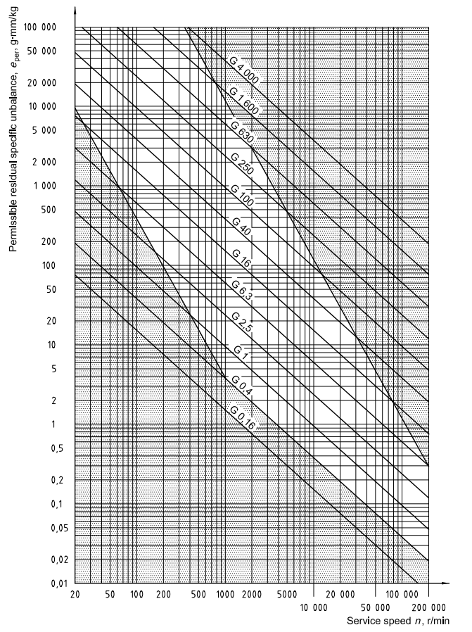
Balanced rotors are essential for most kinds of rotating machinery. Unbalance will create high vibrations causing material defects and reducing the lifetime of a material. In most cases the rotor unbalance is the major problem of vibration, it is related to the first order (= rotational frequency).

We assume, that we consider the so-called rigid rotors, which is true for nearly all practical cases. That means the operating speed of the machine is below 70% of its first resonance frequency. The resonance frequency is the critical speed, where structural resonances cause heavy vibrations. At the resonance, the phase is turning quickly and it would be impossible to make a correct measurement.

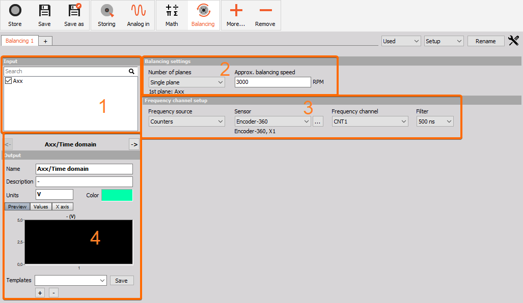
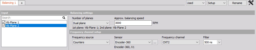
The requirement in terms of sampling rate depends on the first order (e.g. 3000 RPM/60 = 50 Hz required sampling rate 3520 Hz). Also, a precise vibration sensor signal is mandatory.

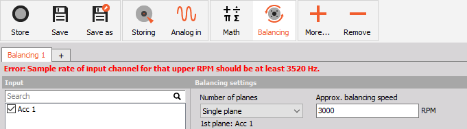Image 1: Required sampling rate for balancing

 

The minimum sample rate is calculated from the balancing speed RPM (Max RPM + 10%) and the maximum order that is selected in the settings (32 is the default). (3000RPM / 60) * 1.1 * 2 * 32 = 3520 Hz

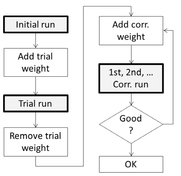
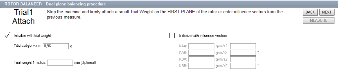
The goal of balancing is to minimize vibrations related to the first order. Basically, it works like this: We measure the initial state, then we add a trial weight of the known mass, calculate the position and mass of a counterweight, remove the trial weight and put the calculated weight on the opposite side, to cancel out the imbalance.

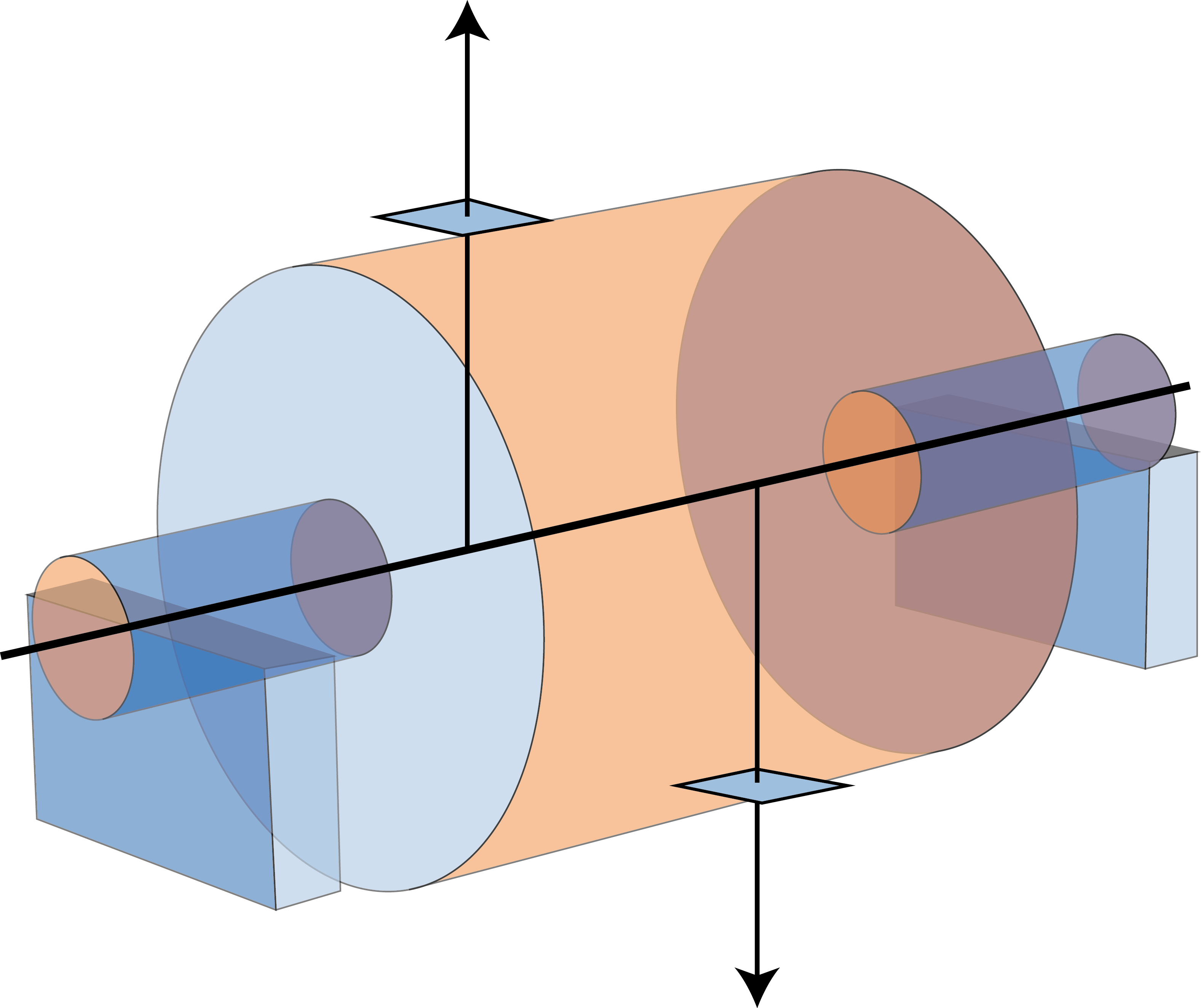
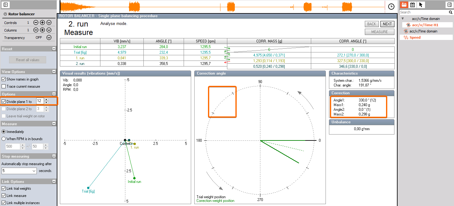
When an unbalance exists, the first order (rotational frequency) can be seen clearly. As shown in the example below, on the rotor exists an uneven distribution of mass.	A correction weight is added (or material is removed) on the opposite side, which cancels out the major part. This procedure can then be repeated until satisfaction.
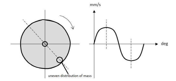Image 2: Uneven distribution of mass	Image 3: Correction weight on the opposite side from uneven distribution of mass

Single and dual-plane balancing

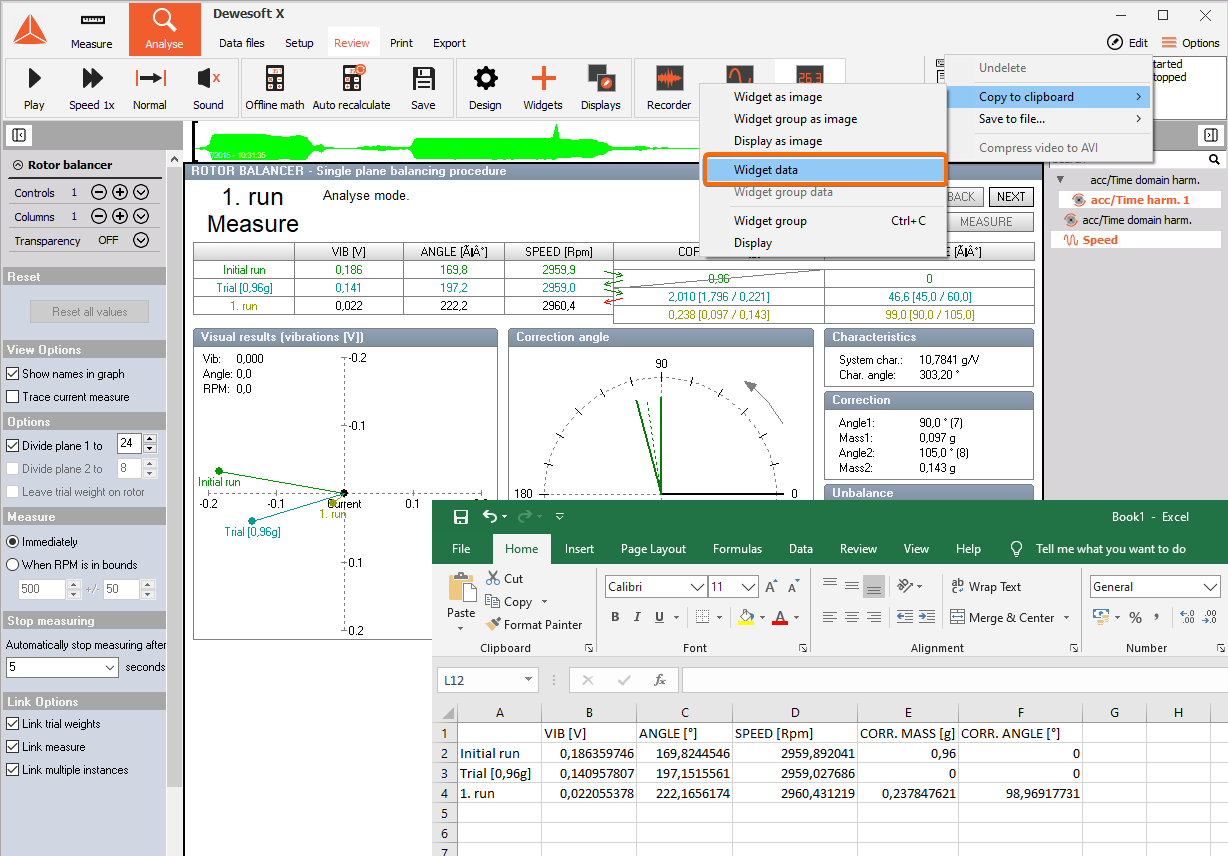
Depending on the machinery, single or dual plane balancing is used. Selecting one plane or two plane balancing generally depends on two factors. One of the factors is the ratio of the length of the rotor (L) to the diameter of the rotor (D). The other factor is the operating speed of the rotor. As a general rule of thumb, we can refer to the table shown below.

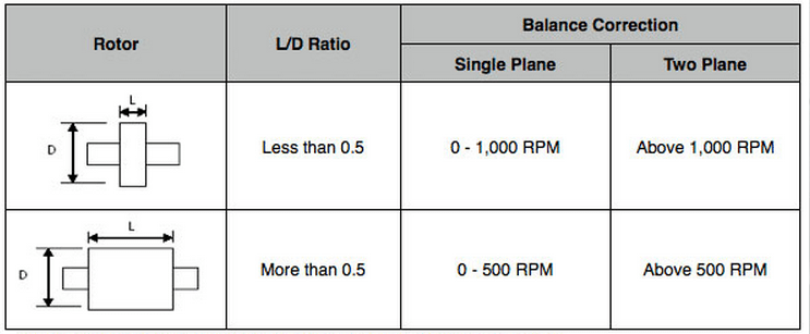Image 4: Selecting between Single and Dual-plane balancing

 

 

The procedure for a single plane or dual-plane balancing will be different, depending on which option is chosen. But basically, the following steps have to be taken:

• initial run
• trial run
• correction run(s)

Needed equipment

• 1 (for a single plane) or 2 (for dual-plane) acceleration sensors
• 1 angle sensor (for measuring RPM and absolute angular position, therefore the angle sensor must have a zero-pulse: rotary encoder with A, B, Z signal, optical tacho probe with the reflective sticker, inductive probe, CDM with zero,...)

The first step of balancing procedure is to do an initial run. The machine has to be run up the operating speed. The vibration velocity is detected. The velocity level and phase angle give together a vector that represents the original unbalance of the rotor. The length of the vector is equal to the vibration amplitude and its direction is given by the phase angle.

Image 5: Initial run at operating speed

 

The second step is to add a trial mass. A trial mass has a known weight and it is fixed at a known radius at an arbitrary angular position on the rotor. The machine is again run-up to operational speed. We get a new vibration velocity level and a new phase angle. These values represent the resultant effect of the initial unbalance and the trial mass.

Image 6: Run with trial mass

 

The tips of vectors V₀ and V₁ are joined by means of the third vector V_T, which is marked so that it indicates the V₀ to V₁ direction. This vector represents the effect of the trial mass alone. A vector is drawn parallel to the vector V_T, with the same amplitude and direction, but starting at the origin.

In the opposite direction to V₀, there is a vector V_C and it represents the position and magnitude of the mass required to counteract the original unbalance.

Image 7: The procedure to determine the vector of unbalance

 

If we assume that the amplitude of the vibration is proportional to the unbalance mass, we get the expression that enables us to find the value of compensating mass (M_COMP).

The position of the mass relative to the position of the trial mass can be determined from the vector diagram.

Now we have sufficient information for the vector diagram with vector lengths proportional to the measured vibration velocity levels.

Image 8: Vector diagram to determine the position of compensating mass

 

The procedure in Dewesoft is guided by the visual control instrument. The flowcharts below show the routines for single and dual-plane balancing. 

Single plane balancing procedure

Image 9: Single plane balancing procedure

 

Dual plane balancing procedure

By adding the correction weights for both planes at the same time, we save one additional step.

Image 10: Dual-plane balancing procedure

 

A frequency analysis of the vibration signal also guides us in the selection of the best parameter for measuring the vibration. The vibration can be measured in terms of:

• acceleration,
• velocity,
• displacement.

The three curves have different slopes, but the peaks in the spectrum occur at the same frequencies in each case. The same information about the vibration levels is contained in each curve, but the way the information is presented differs considerably.

The parameter selected for vibration measurement is usually the one with the flattest curve (the most horizontally aligned spectrum). This parameter requires the smallest dynamic range in the measuring instruments, so the signal-to-noise ratio is higher - the parameter with the flattest curve is velocity and this is also the parameter that is most frequently used.

The advantage of Dewesoft dual-core technology is the wide dynamic range and can detect very small or very high vibrations at the same time. So there is no need to select the parameter with the smallest dynamic range when performing balancing with Dewesoft equipment. But the velocity is the most commonly chosen parameter because it is used in most standards.

Image 11: Vibration parameters

 

Unbalance is a result of uneven distribution of mass, which causes the machine to vibrate. The vibration is produced by the interaction of an unbalanced mass component with the radial acceleration due to the rotation, which together generates a centrifugal force. Since the components rotate, also the force rotates and tries to move the rotor along the line of action of the force.

Static unbalance

Static unbalance is an eccentricity of the center of gravity of a rotor, caused by a point mass at a certain radius from the center of rotation.

An equal mass placed on the opposite side (180 deg) will balance the rotor.

Image 12: Static unbalance

 

Couple unbalance

A couple of unbalances may be found in a rotor whose diameter is less than 7 to 10 times its width. In the case of a cylinder, it is possible to have two equal masses placed symmetrically about the center of gravity, but positioned at 180° from each other. The rotor is in static balance (there is no eccentricity of the center of gravity), but when the rotor turns, the two masses cause a shift in the inertia axis, so that it is no longer aligned with the rotation axis, leading to strong vibrations.

The unbalance can only be corrected by taking vibration measurements with the rotor turning and adding correction masses in two planes. Couple unbalance rotor is stationary, the end masses balance each other. However, when it rotates, a strong unbalance is experienced.

Image 13: Couple unbalance

 

Dynamic unbalance

Dynamic unbalance is a combination of static and couple unbalance and is the most common type of unbalance found in rotors. To correct dynamic unbalance, it is necessary to make vibration measurements while the machine is running and to add balancing masses in two planes.

Image 14: Dynamic unbalance

 

The channel setup of the plugin in Dewesoft is very intuitive and simple to use.

The plugin is split into the following sections:

1. 1.) Vibration inputs for planes - here you select your acceleration sensor. They should be mounted close to the shaft (e.g. on the bearing).
2. 2.) Balancing settings - specify the method of balancing (single or dual plane) and the operating speed of the machine.
3. 3.) Tacho input - a speed sensor with a zero pulse is needed (e.g. encoder, tacho probe with 1 pulse/rev, CDM with zero...).
4. 4.) Output channels - get a quick preview of the signals (time domain of the first order and speed), useful for checking if the tacho input is working correctly.
5. 
   

Image 15: Channel setup of the balancing module

 

When you have set up the balancing module in channel setup, there is an automatically generated display called Balancing in Measure mode.

Image 16: Auto-generated balancing measurement screen

 

It is basically a visual control instrument (the RotorBalancer), which will guide you step-by-step through the procedure. On the top you see the current step, with an explanation which action has to be taken, on the right, there are the interactive buttons Back, Next, Measure.

The table with name of runs, vibration amplitude, angle and RPM is empty at first and will fill with the results after each step. The polar plot on the left shows the vibration levels (amplitude and angle) of each run (the unit depends on the input, mm/s, or mm/s² or g is usual).

The graph for the correction angle on the right helps when it comes to mounting the correction mass.

On the right column, you can see system characteristics and the overall unbalance. The correction weight and angle are also displayed here.

Let's make a practical measurement example on a machine. Here we will show a dual-plane balancing procedure on a grinding machine. The planes have been modified for demo purposes, so we can mount screws as unbalance/trial/correction weights.

A 360 pulses encoder is installed on one side, two acceleration sensors are mounted (one on left and one on right bearing; only one shown on photo) and connected to a SIRIUS measurement instrument.

Image 17: Dual-plane balancing demo equipment

 

In the channel setup of the balancing plugin, we need to specify the acceleration sensors of both planes for input (plane1, plane2), as well as the "dual plane" procedure.

Image 18: Dual-plane balancing channel setup

 

The machine is an asynchronous one, so it will run with approx. 3000 rpm. The procedure will be done according to the dual-plane step-by-step procedure.

Initial run

Some weights have been mounted before at random angular position to simulate a bigger unbalance. Other than that, we leave the machine unmodified and just start it. When we have reached operating speed, click on Measure.

The button will change to a stop button with running dots, showing that the measurement is in progress. After that, the button will change back to Measure again, meaning that you also can repeat the measurement if something was wrong.

Image 19: The measure button changes to stop button

 

Image 20: Initial run

 

Trial 1

Now we have to mount trial weights sequentially, first for the Plane #1.

We apply a screw of known mass at a random position. Please remember to mark this position, as it will be the reference (= 0 deg) angle for the correction mass in future steps!

Then we enter the trial weight mass. 

Image 21: Attaching a trial weight on the first plane

 

 

Start the machine and perform the Trial 1 measurement.

Note the warning below in red, showing that a bigger trial weight will give a better result. So, the difference with/without trial weight is too small in our example and we need to mount a bigger trial mass.

Image 22: Trial measurement 1

 

Trial 2

Stop the machine, remove trial weight #1, and mount a known trial weight on plane #2. Then enter the mass in the plugin.

Image 23: Attach trial weight on the second plane

 

Then run the machine again and collect the data.

Image 24: Trial measure 2

 

After the measurement we can already see the calculated correction weights on the right side:

• Plane 1: 0,599 g at 101,2°
• Plane 2: 2,487 g at 345,4°

When you click on Next, you will see a draft of the correction weight positions. Trial weight position is 0° and the angle is positive in direction of movement.

Image 25: First correction attached

 

 

Correction run

Now remove the trial weight #2, before you continue.

Then mount the correction weights and start the measurement.

In our example the result for both planes has been improved, the 1.run vector has a smaller amplitude than the Initial run vector. Actually, it worked better for the first plane, so we would have to go for a second corrective run.

Image 26: First run after the measurement

 

The weights for the next run are already suggested. As you can see, the mass is already significantly lower. It should decrease further with each following run.

View options

The Show names in graph option as seen in previous screenshots add the names to the vectors of each run, e.g. Initial run, Trial, 1.run, Current...

Image 27: Option Show names in graph

 

To check if amplitude and phase are stable at the operational speed, it may be helpful to trace the current vector over the change of RPM, this can be done by selecting Trace current measure.

Image 28: Trace current measure option

 

Weight splitting

When you have a rotor/plane with a certain number of slots/blades/holes, where the weights can be mounted, it would be much easier just to know the position number and split the weights instead of the absolute angle.

This can be done by selecting Divide plane xx to xx from the properties. In our example we have a plane with 24 holes, so we mount weights in positions 3 and 4.

After adding the trial weight, and before adding the correction weight, there is a possibility to check the option Leave the trial weight on rotor. This is a nice feature for any situation, where removing the trial weight is a too big effort.

Image 29: Divide plane option

 

Measure options

During the procedure, when you click the Measure button, the data is averaged over the time shown below (Automatically stop measuring after xx seconds).

To ensure, the measurement is performed always at the same RPM, you can additionally set a target value and boundary.

Image 30: Measure immediately or when RM is in bounds

 

Link multiple instances

Sometimes when the amplitude and phase of the signal are not stable you have to find a different location for mounting the sensor, to get a better signal.

To save time, you can mount multiple sensors and measure them at once, and then decide which signal to take. The whole procedure is the same, but you only need to operate one VC (visual control), all the other instruments will follow, of course providing different results.

Image 31: Link multiple instances

 

Therefore, in Measure mode please check the Link options (left lower part).

The Rotor Balancer visual control can be picked from the instrument toolbar in Design mode. The channels Speed and xxx/Time H1 have to be assigned to it.

image 32: Link options

 

Which of the results should now be chosen for the correction?

• The one where amplitude and phase are stable.
• The one with the smallest influence vector.

The influence vector describes the relation between the vibration pattern changes on a specific mass change. 1g/mm/s tells us that 1g will change the vibration level of first-order for 1mm/s. If the influence vector is 0,5g/mm/s we only have 0,5g to get the same vibration change. So we should carry on balancing where a small trial mass will give us a high vibration signal. So the unbalance is clearly seen on the structure and not damped. So, we should carry on where the influence vector is 0,5g/mm/s!

Image 33: System characteristics

 

Initialize with system characteristics

If Balancing was already done on a particular shaft, and the system characteristic is known, a trial weight run is not necessary once again; the system characteristics parameters can be entered manually instead, to get the correction mass calculated immediately.

This could be used if a shaft is balanced multiple times at a certain interval.

The system characteristics describe the relationship between mass and vibration.

If a previous setup was stored and loaded again, the system characteristic was stored in the balancing visual control, too. Now it could be entered manually or RESET ALL VALUES could be pressed.

Image 34: Reset all values

 

After that is done, the procedure will start on Enter Sys.Char.. After the Initial run, instead of a trial mass, the VC will automatically overwrite the previous system characteristics.

Image 35: Initialize with system characteristics

 

To rebalance a system with the use of the previous system characteristics value, the following requirements have to be met:
- the rotor was previously balanced with a trial mass
- the rotor characteristics have not changed
- the position of the first trial mass must be known (mark on shaft/disc)
- if an optical tacho probe was used: the reflective sticker (trigger zero signal) must stay at the same position
- an optical tacho probe and vibrations sensor must have the same angle relative to each other
- the same balancing speed (RPM)

Acceleration to velocity calculation

In Dewesoft, it is possible to directly integrate from acceleration to velocity in the channel setup. Just activate the checkbox, and set the according to filter (recommendation 4th order, 4 Hz). Due to the mathematical integration, there is a constant added to the result, which must be filtered out. If the filter order is too high and the Low frequency is too low, you can see a slow-moving offset, even if there is no signal at the input! - In this case please adjust the filter properly, use an FFT to check for your lowest interesting frequency.

Image 36: Acceleration to velocity

 

Removing mass

Instead of adding the correction masses, mass can be also removed from the rotor (e.g. by grinding). You just have to apply it on the opposite side (+ 180°).

During the whole process, all raw data is stored, see below the orange curve (vibration time domain data) in the overview instrument. Additionally, when we reload the data file in Analyse mode we will have angle and mass data of all runs (initial, trial, correction).

As expected, the last run has the smallest amplitude (=less vibrations), which means our rotor has been balanced successfully.

Image 37: Analyzing the balancing datafile

 

The RotorBalancer visual control shows the polar plot with the vectors of each run, in the table you can see the correction masses and angles for each run.

Balancing only works live in Measure mode!

After we had successfully balanced a rotor and collected the data, you can export the data of all runs.

Therefore click on the RotorBalancer visual control element to be active, then select Edit Copy to clipboard Widget data.

Then you can paste the data e.g. to Excel, as shown below.

Image 38: Copy widget data to the clipboard

 

Please take a look at the following video for an easier understanding of how balancing procedure is done with Dewesoft hardware and software.

Experimental evaluation of the balance quality requirements is often carried out for mass production applications. Tests are commonly performed in situ. The permissible residual unbalance is determined by introducing various test unbalances successively in each correction plane, based on the most representative criterion (e.g. vibration, force, noise caused by unbalance).

In two-plane balancing, if no tolerance planes are used, the different effects of unbalances with the same phase angle and of that 180° apart shall be taken into account.

In the image below, there is guidance for balance quality grades for rotors in a constant (rigid) state.

Image 39: Guidance for balance quality

 

In the image below, there are shown permissible residual specific unbalance based on balance quality grade G and service speed n. The picture contains generally used areas (service speed and balance quality grade G), based on common experience.

The white area is the generally used area, based on common experience.

Image 40: Permissible residual specific unbalance

 

This section should help to find quick solutions for known problems.

Amplitude and phase not stable

The amplitude and phase must be stable to get a reliable result. For verification, you can use the option “Trace current measure”. The curve must be stable and not jump at the operational speed. If it does jump, there can be several reasons.

• Vibration signal is too small/noisy. -> Please mount the accelerometer on a different position.
• RPM signal is not stable. -> Check tacho signal and readjust trigger level.
• Balancing is done close to or on the structural resonance frequency. The operating speed is close to the resonance frequency of the structure. Therefore, the phase is changing for 180deg. If first order falls on such a resonance, a small frequency change (rpm change) will create a big phase change. Below a modal test has been done on a structure. The machine is operated at 50 Hz (3000 RPM), where amplitude and phase are stable, you will get a good result. Please compare to the region of around 300 Hz. There is a big phase jump, where it would be impossible to get a stable initial run vector.

Rotor balancer visual control not found

• The visual control called “RotorBalancer.vc” has to be located in the Addons folder of your Dewesoft X installation (e.g. D:\Dewesoft\Bin\X2\Addons). If it's not there, please restart the Dewesoft X Full installer, select “Modify” and activate at least the Plug-ins and Visual controls of the Add-ons section. 
• After you have ensured, the plugin exists in the correct folder, please check under Settings and do the “Register plugins”.