Modal test and analysis are used to determine structural modal parameters, such as modal frequencies, damping ratios, and mode shapes. The measured excitation and response (or only response) data are utilized in modal analysis, and then dynamic signal analysis and modal parameter identification are processed. Modal test and analysis techniques have been developed for more than three decades, and a lot of progress has been made. It has been widely applied to the engineering field, such as the dynamic design, manufacture and maintenance, vibration and noise reduction, vibration control, condition monitoring, fault detection, model updating, and model validation.
Modal test and analysis is needed in every modern construction. The measurement of system parameters, called modal parameters, are essential to predict the behavior of a structure.
These modal parameters are also needed for mathematical models. Parameters like resonance frequency, structural damping, and mode shapes are experimentally measured and calculated.
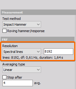
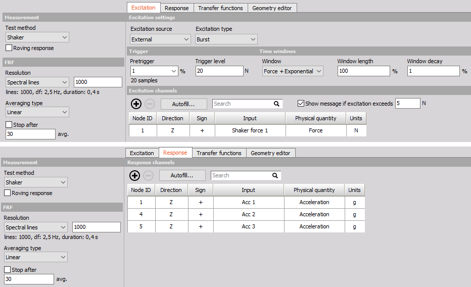
The Dewesoft Modal Test module is what you use when performing structural dynamic test measurements of objects. The Modal Test provides calculated FRF functions (amplitude and phase) over a certain frequency range.
The Dewesoft Modal Analysis module is used after the modal test data acquisition in order to estimate high quality modal models.
The Modal Analysis module uses the results from Modal Test, e.g. FRFs, to estimate modal parameters (resonance frequencies, damping ratios and mode shapes)
The Dewesoft Modal Test module also provides tools to determine modal parameters as well, but these tools only apply for simple structures, having lightly damped and well separated modes.
Dewesoft Modal Analysis is required to obtain valid modal parameters for complex structures, having multiple resonance frequencies being closely spaced or with heavy damping.
The Dewesoft Modal test module is included in the Dewesoft X DSA package (along with other modules e.g. Order tracking, Torsional vibration, etc.).
The Dewesoft Modal Analysis module comes as a separate license and is not included in the DSA package.
With the small, handy form factor of Dewesoft data acquisition instruments (DEWE-43, SIRIUSi), it is also a smart portable solution for technical consultants coping with failure detection.
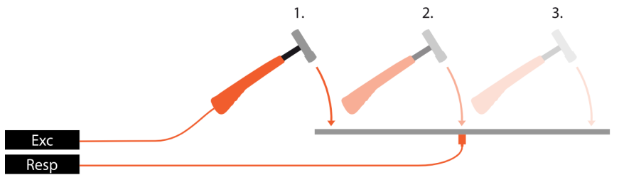
Let's assume there is a mechanical structure to be analyzed. Where are the resonances? Which frequencies can be problematic and should be avoided? How to measure that and what about the quality of the measurement? Probably the easiest way is exciting the structure using a modal hammer (force input) and acceleration sensors for the measurement of the response (acceleration output). At first, the structure is graphically defined in the geometry editor.
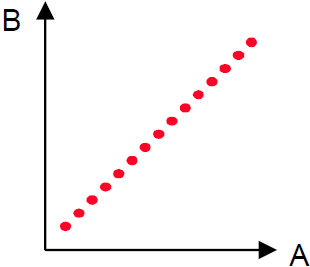
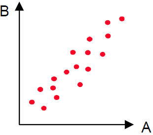
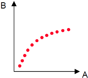
Then the points for excitation and response are selected and linked to the defined geometry. The test person knocks on the test points while the software collects the data. Next to extracting phase and amplitude, it is possible to animate the structure for the frequencies of interest. The coherence acts as a measure for the quality. The modal circle display widget provides higher frequency precision and damping factors for modes on simple structures. For additional analysis and for handling complex structures you continue using the modal analysis module.
If desired the data can be exported to several file formats like the widely used UNV format.
A used example of modal test and modal analysis are shown below:
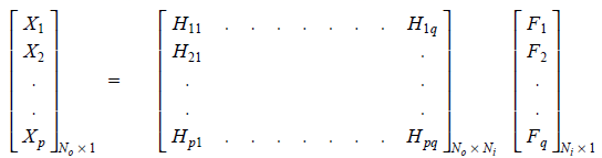
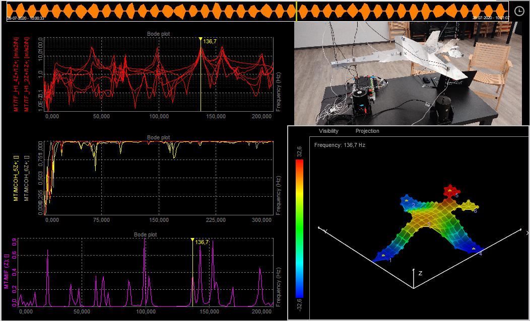
 Example of a Modal Test application.
Example of a Modal Analysis application.
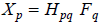
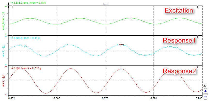
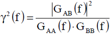
 Image 1: Explanation of frequency response function