Example II - Lane departure
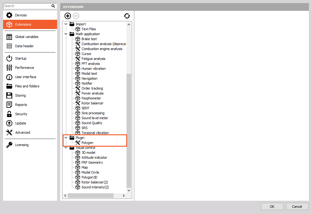
In this chapter, you will learn how to create a basic setup to monitor the distance between the lane line and the VUT. Here we will use a Vehicle simulation plugin, layers from Vransko proving ground and Rimac Nevera model, all available for downloading here.
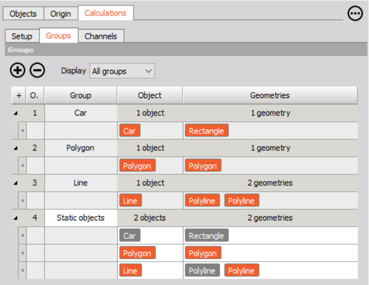
For this task using Polygon, you will learn to perform a simple ‘Line assist warning test’. Origin will be setup with 2 Points that are separated 85,5 m in X direction:
P1 46° 14.579883' N 14° 58.407817' E (0, 0)
P2 46° 14.533803' N 14° 58.410700' E (85.5, 0)

Now the Straight Line should be added that will represent the line on the middle of the track. Because of the width of the line in real life, what is the most convenient way to recreate it in a virtual environment? We have to use a rectangle with defined width (0.15 m) and length (120 m).
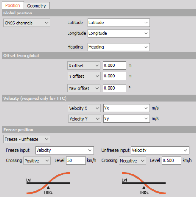
The object with Vehicle geometry should be added and assigned a Navigation channel from Vehicle simulation. In the Vehicle simulation plugin type in coordinates (46° 14.579883' N 14° 58.407817' E Heading - 357 ). Now the Vehicle is on the Vransko proving ground.
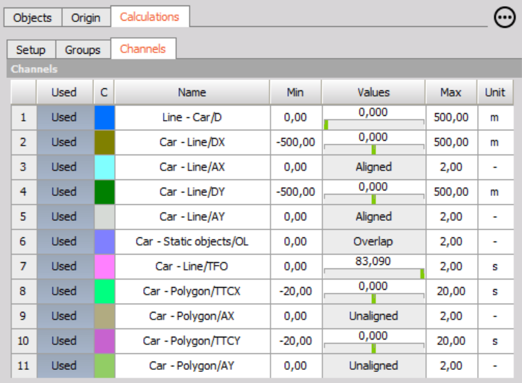
Add the proper calculation that will measure the shortest distance between the vehicle and this line.
When you enter measure mode, and you open the Polygon display, you have an option to add layers.
Press edit button and then add a local layer from folder Vransko, which you downloaded on the start of this task.
You have uploaded layers, now also load a model. Dewesoft supports a lot of different model formats (.amf, .glb, .gltf, .obj, .stl, .stp, etc.) but we suggest .obj or . gltf. On the link you have also downloaded Nevera.obj and Nevera.mtl files. Be sure that both are in the same folder before loading the model in DewesoftX.
When the window opens, click ‘Load new model’ and then the Nevera model should be properly loaded.
When a model is Loaded, you can define size and center of the model. You can check ‘Keep original aspect ratio’ or define every dimension by yourself. Here you will define only the Length to 4,75 m and define the Centre of the model as shown on the image below.
You can now select Nevera as a 3D model in Polygon to drive around the track.
Now in the measurement screen add an Indicator lamp, that will turn red, if the calculated distance is less than 5 cm. Also add additional lamp for the Overlap calculation.
With this setup, you can now perform Lane assist test and monitor the distance between the VUT and the lane. In real measurement, you can also add camera and/or microphone in combination with positioning data to monitor the functionality of the system.
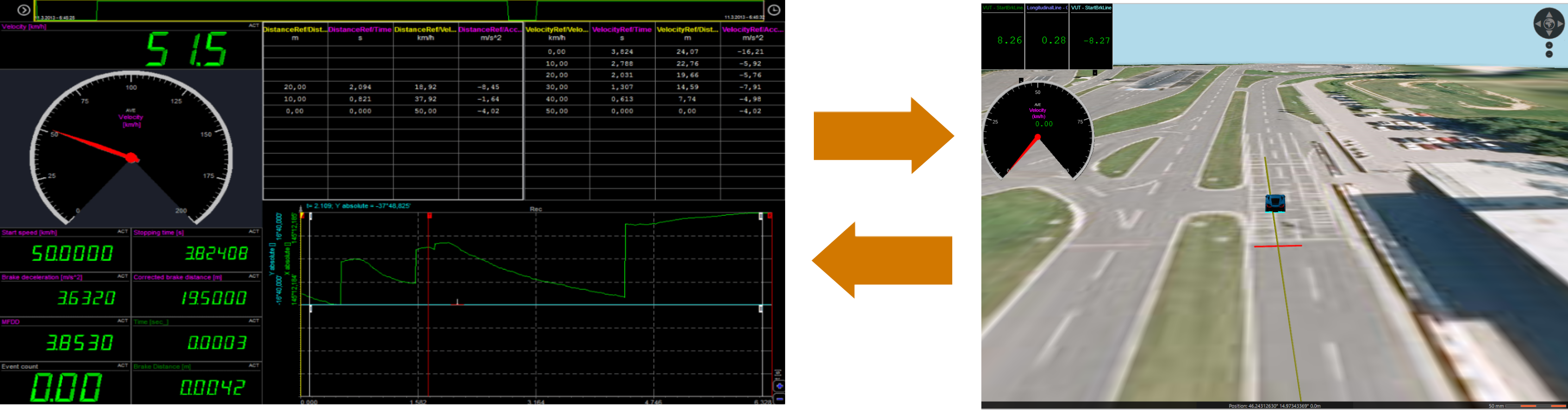 Image 1: Measurement together with 3D visualization