Reference Curves For Signal Comparison

With the reference curves, we can compare different types of signals (time domain, frequency domain) to the reference signal and see whether our signal is above or below the reference limit.

The reference curve is defined by a user. With the reference curves, we can compare different types of signals (time domain, frequency domain) to the reference signal and see whether our signal is above or below the reference limit.

Available reference curves in Dewesoft X are:

  • time reference curve,
  • XY reference curve,
  • frequency domain reference curve, and
  • vector reference curve.

Reference curve preview
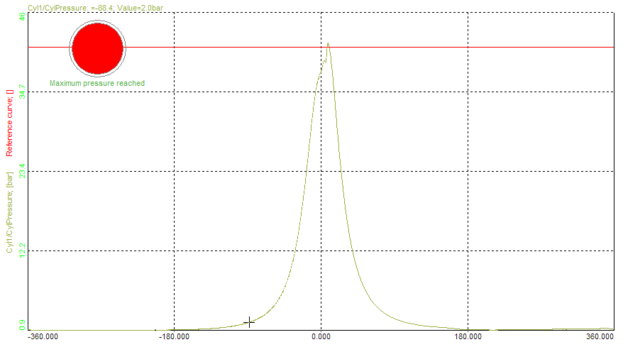
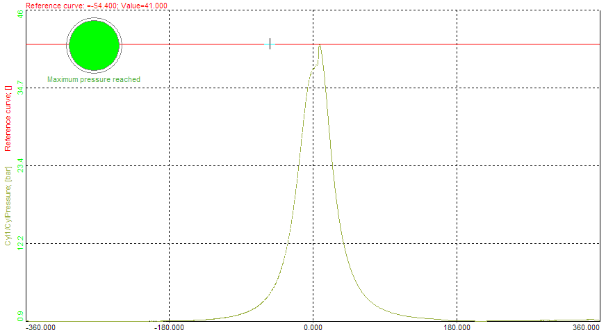
Image 1: Reference curve example

With Time reference curve we define the reference curve in the time domain, displayed on the recorder. The time reference curve is used for monitoring the time domain data. The time reference curve can be added under math functions Add math -> Time reference curve.

Image 2: Add the Time reference curve 


Time based Reference curve

The Time based reference curve is useful for defining a curve in time as a reference during a certain test, which has to follow a certain protocol. Let's say we have a test where we need to accelerate to 100 km/h in 10 seconds, drive constantly for 10 seconds, and decelerate to 0 km/h in 10 seconds.

We can define each curve starting criteria. If the Start condition channel is not defined, the curve will start at the beginning of the measurement. Maybe it would be nice to define the start of the test on a channel that measures vehicle velocity, but then we have to define the limit on which the measurement will Start if value is above (this field appears only when Start conditional channel is selected - default = ). In our example, we could enter for example 2 km/h.

The next step is to define the Number of points and the points themselves in the list. In our case we would have four points, so we enter this in the field.

Image 3: Time based reference curve 


Single value based Reference curve

A single value based reference curve can be understood as a sort of non-linear scaling. We need to define a First reference channel, Number of points, and a table with the values of reference and output channel.

So in the example on image 4, if the input channel will be 3, the output value will be 5. The values will be interpolated in between the points. So if the input is 2.5, the output will be 3.5. If the value is below or above the lowest or highest point, data will be extrapolated from the two lowest or highest points. If we have 0 at the input, we will have 0 at output. If we have 5 at the input, we will have 11 at the output.

On the upper right, you will have previewed diagram of your inputs.

Single value based reference curveImage 4: Single value based reference curve
"Single value based" option was removed from Time reference curve setup from Dewesoft X3 SP12 - Release notes.
Substitute is to use Scaling math and configure "Input value" column as "Ref. value" column in old setup.


Dual value based Reference curve

Dual value based reference curve has two inputs: First reference channel and Second reference channel. We can imagine as the tridimensional surface of reference points X and Y are two reference channels while the Z is defined points. We need to define first the channels and the Number of points for each channel.

Then we need to enter the reference values in the list. Display on the right upper part if the Reference curve setup window now shows the curve.

Dual value based reference curveImage 5: Dual value based reference curve 


A good example of using a dual reference curve is to define the limit oil pressure referenced to RPM and the oil temperature.

From data file Reference curve

The time reference curve can be imported from another data file.


From data file reference curveImage 6: Reference curve From data file


Let's say we have a test where we need to accelerate to 100 km/h in 10 seconds, drive constantly for 10 second and decelerate to 0 km/h in 10 second.

In our example, we can enter the start condition for example 2 km/h. The table below shows how our vehicle should behave.

Point numberTime [s]Velocity [km/h]
1st02
2nd10100
3rd20100
4th300


The next step is to define the number of points and the points themself. In our case, we have 4 points.


Image 7: Define the number of points and the points themself 


We can display our time reference curve on the recorder. Then we can use the Formula Math channel, to see if we are above or under our reference:

if('Vehicle_Acc'>'Reference5',1,0)


This formula will give you a value of '1' if our signal from the vehicle is above the reference curve and '0' if our real signal is below the limit.

Monitoring point will change its color as the real signal will go above the reference curveImage 8: Monitoring point will change its color as the real signal will go above the reference curve


The XY reference curve math module provides the reference curve for the XY recorder. The XY reference curve can be added the same as the Time reference curve was, under Add math -> XY reference curve.

When you open the setup for the XY reference curve, the window shown on image 9 will open.

Image 9: XY reference curve setup

After choosing the input channels for the X and Y channel, we need to set the number of points for the XY reference curve. The reference points can be entered value by value or transferred with the copy-paste function. Copy button copies all the points to the clipboard in a tab-delimited style, so it can be easily pasted to any spreadsheet software. Also, the values can be copied from other spreadsheets with the Paste command, where the data has to be tab-delimited and each line should be terminated with carriage return/line feed character.

For example in the following picture of MS Excel, we chose the data range and selected Copy, afterward, the data can be easily pasted into Dewesoft X.

Image 10: Easily Copy-Paste values to, or from MS Excel 

There is another advantage of the reference curve. The output channel (Status in our case) gives a value of 1 when the XY curve crosses the reference curve. This can be used for trigger criteria or for counting of events (with ECNT function in formula editor).

Image 11: The output channel gives a value of 1 when the XY curve crosses the reference curve

In the example below, we have two Eddy current proximity probes that measure proximity. While placing the probes around the shaft, we can see the movement of the shaft. In the reference curve setup, we defined the rectangular, with maximum allowed movement.

Define the rectangular with maximum allowed movementImage 12: Define the rectangular with maximum allowed movement


With displayed XY reference curve in the XY recorder, we can monitor the movement of the shaft and if it stays inside the allowed borders.

Image 13: Monitoring the shaft movement

The FFT reference curve math module provides the reference curve for the FFT display. It can be used for displaying the reference on FFT screen and also to provide a math output channel which goes high when the levels are exceeded.

FFT reference curve can be added under the Math section, Add math -> Frequency domain reference curve.

In the channel setup, we define the maximum number of lines, window type, and overlap.

Image 14: FFT reference curve 


These values will be used for the calculation of the FFT spectrum. Then we define the limits - limit table. They can be entered value by value or from current data.

Get current data means that current FFT (in the setup screen) will be taken as the reference. We can define some offset to that reference (with up/down and left/right arrows button). Similar to the FFT trigger it will raise/widen the current transfer curve.

Image 15: Get current data

The FFT reference curve can be used in FFT display to show some reference lines, while the output channel (named Status in the screenshots) can be used for displaying either if the current data is above or below the defined reference.

Image 16: Reference curve on FFT

Let's take an example of using the tuning fork. With the reference curve, we can check if the tuning forks are working correctly. The frequency of tuning fork is approximately 440 Hz. We create a reference curve, with allowed amplitude and frequency range.

Image 17: Create a reference curve, with allowed amplitude and frequency range 


We add an FFT display, select the channel (Tuning fork) and display the FFT reference curve. The FFT reference curve can be obtained during the measurement, with the Get current data option.

During the measurement, we can also observe the time signal on the recorder and the FFT of the signal as it is shown on image 18. If the FFT signal from the tuning fork (green) is under the FFT reference curve (red) we can conclude that the tuning forks are working properly.

 Preview the FFT diagram of tuning forks and apply the FFT reference curveImage 18: Preview the FFT diagram of tuning forks and apply the FFT reference curve

In vector reference curve we define the reference curves for the input channel, which is usually an array (FFT data, ...).

Image 19: Vector reference curve setup 


The reference curve type can be selected from:

  • lower (define the lower limit),
  • upper (define the upper limit), and
  • lower & upper (define the lower and upper limit).

With linear interpolation, the program will draw a direct line between the two neighborhood points. It will give a smoother transition between points on the curve.

Image 20: Impact of the linear interpolation  

Check signal bounds will create an additional output channel which will output '1' when the input is higher than the reference curve and will output '0' when the input is below the reference curve

Axes settings can be selected from:

  • linear,
  • logarithmic,
  • 0 dB (dB reference will be set from the range of the first channel),
  • Noise dB (the reference value is 20 uPa), and
  • ref. dB (user enters the reference value).

Image 21: Axes settings 

Next, we define the points in the limit table. We can define the points manually or copy/paste if from an external program.

Rename the channels with the click on the icon in the top right corner and selecting the Change axis name/unit option.

Change namesImage 22: Change names

When we paste the data from an external program (e.g. Excel) we have to be careful to write the right names for the axis.

Create a reference curve math with add Math -> Vector reference curve.

Open the settings for the vector reference curve and select the channel that will be used for checking the level - we use CylPressure.

Linear interpolation will give a smoother transition between points on the curve. Check signal bounds will create an additional output channel which will output 1 when the input is higher than the reference curve and will output 0 when the input is below the reference curve.

The reference curve is defined with a table. The first column is the crank angle (X) axis, and the second column the amplitude of the reference (Y) axis. In this first example, we have defined only two points with a value of 41 (bar).


Image 23: Set the table for CylPressure channel 

We have added a CA scope and selected the cylinder pressure signal and reference curve for display. An indicator lamp was also added and the output channel from the vector reference curve assigned to it. When the pressure is above the reference curve the indicator lamp will turn red, otherwise, it stays green. The output from the channel goes from 0 to 1, when the reference axis is crossed.


Image 24: Monitoring CEA scope with cylinder pressure signal and the reference curve - Maximum pressure was reached


Image 25: Monitoring CEA scope with cylinder pressure signal and the reference curve - Maximum pressure is not reached yet


We can modify the simple reference curve. It is also very easy to create a reference curve from a recorded pressure signal. For this, we need some datafile with the pressure signal that will be used as a reference.

First, we add Basic statistics inside the Math section.

We open the basic statistics setup and select the pressure channel from the combustion analysis module (combustion analysis must be added in order to have a crank-angle domain instead of time-domain). Maximum should be selected to get the maximum value of all the cycles and under calculation type time based and single value.

Image 26: Setup the basic statistics 

When we add this new channel on the CA scope we see that we get the maximum value of pressure from all the cycles.

Image 27: On the CEA scope you are able to see the maximum value of pressure from all the cycles 

Now we need to make an offset curve that will be used as a trigger. As an example, we will make a curve that will trigger the vector reference curve output channel when the maximum pressure is above 110%.

We create a new formula in the Math module where we multiply the previous basic statistics channel with 1.1.

'ABS MAX Pressure'*1.1


The next step is to display only the last created formula on the CEA scope and copy the data to the clipboard.

Image 28: Copy CEA scope data 

We open again the vector reference curve setup and simply paste the values.

Image 29: Paste CEA scope data as the vector reference curve 

It is also possible to reduce the number of points for the reference curve in Excel.

Copy the data to excel and use the formula =OFFSET(Sheet2!A$1,(ROW()-1)*100,0) to output only every 100th line. This will make modifying the refence curve much easier since there will be only 37 points left instead of 3600.

Image 30: Reference curve from MS Excel