Sound power measurement

Sound is actually a pressure wave - a vibration that propagates as a mechanical wave of pressure and displacement.

Sound propagates through compressible media such as air, water, and solids as longitudinal waves and also as transverse waves in solids. The sound waves are generated by a sound source (vibrating diaphragm or a stereo speaker). The sound source creates vibrations in the surrounding medium. As the source continues to vibrate the medium, the vibrations propagate away from the source at the speed of sound and are forming the sound wave. At a fixed distance from the sound source, the pressure, velocity, and displacement of the medium vary in time.

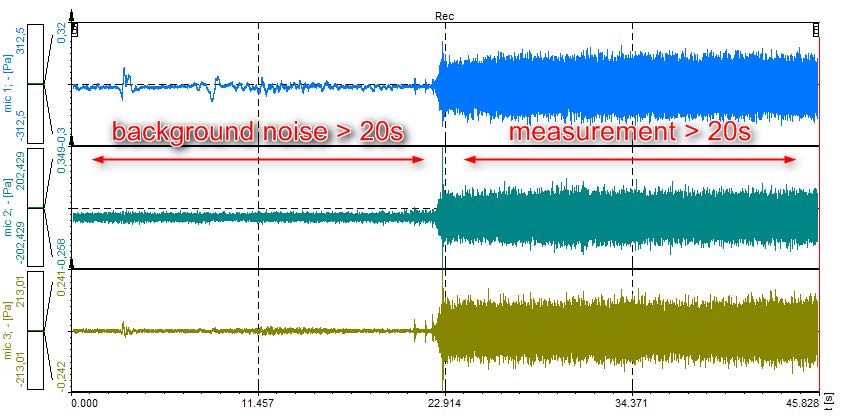
Image 1: Sound is a pressure wave - a vibration that propagates as a mechanical wave of pressure and displacement

 

Sound pressure

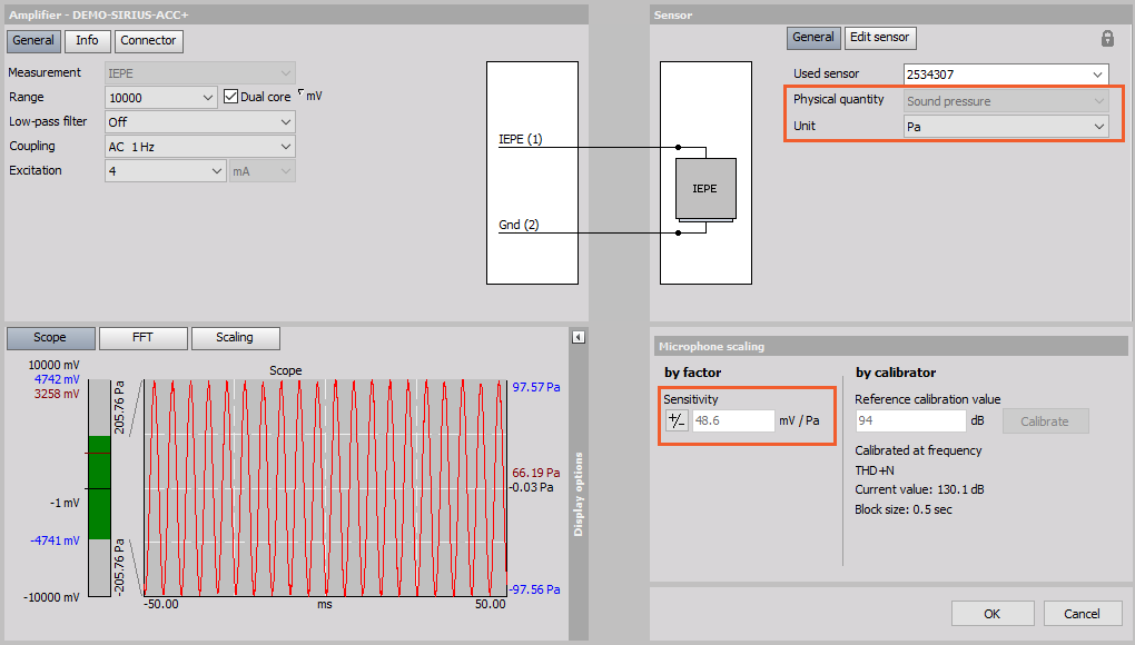
Sound pressure or acoustic pressure is the local pressure deviation from the ambient (average, or equilibrium) atmospheric pressure, caused by a sound wave. In air the sound pressure can be measured using a microphone, and in water with a hydrophone. The SI unit for sound pressure p is the pascal (symbol: Pa).

Sound pressure level

Sound pressure level (SPL) or sound level is a logarithmic measure of the effective sound pressure of a sound relative to a reference value. It is measured in decibels (dB) above a standard reference level. The standard reference sound pressure in the air or other gases is 20 µPa, which is usually considered the threshold of human hearing (at 1 kHz). The following equation shows us how to calculate the Sound Pressure level (Lp) in decibels [dB] from sound pressure (p) in Pascal [Pa].

\( L_{p} = 10\cdot log_{10} \left(\frac{p_{rms}^{2}}{p_{ref}^{2}}\right) = 20\cdot log_{10}\left(\frac{p_{rms}}{p_{ref}}\right) \)

where \( p_{ref} \) is the reference sound pressure, and \( p_{rms} \) is the RMS sound pressure being measured.

Most sound level measurements will be made relative to this level, meaning 1 pascal will equal an SPL of 94 dB. In other media, such as underwater, a reference level \( p_{ref} \) of 1 µPa is used.

The lower limit of audibility is defined as SPL of 0 dB, but the upper limit is not as clearly defined. While 1 atm (194 dB Peak or 191 dB SPL) is the largest pressure variation an undistorted sound wave can have in Earth's atmosphere, larger sound waves can be present in other atmospheres or other media such as underwater, or through the Earth.

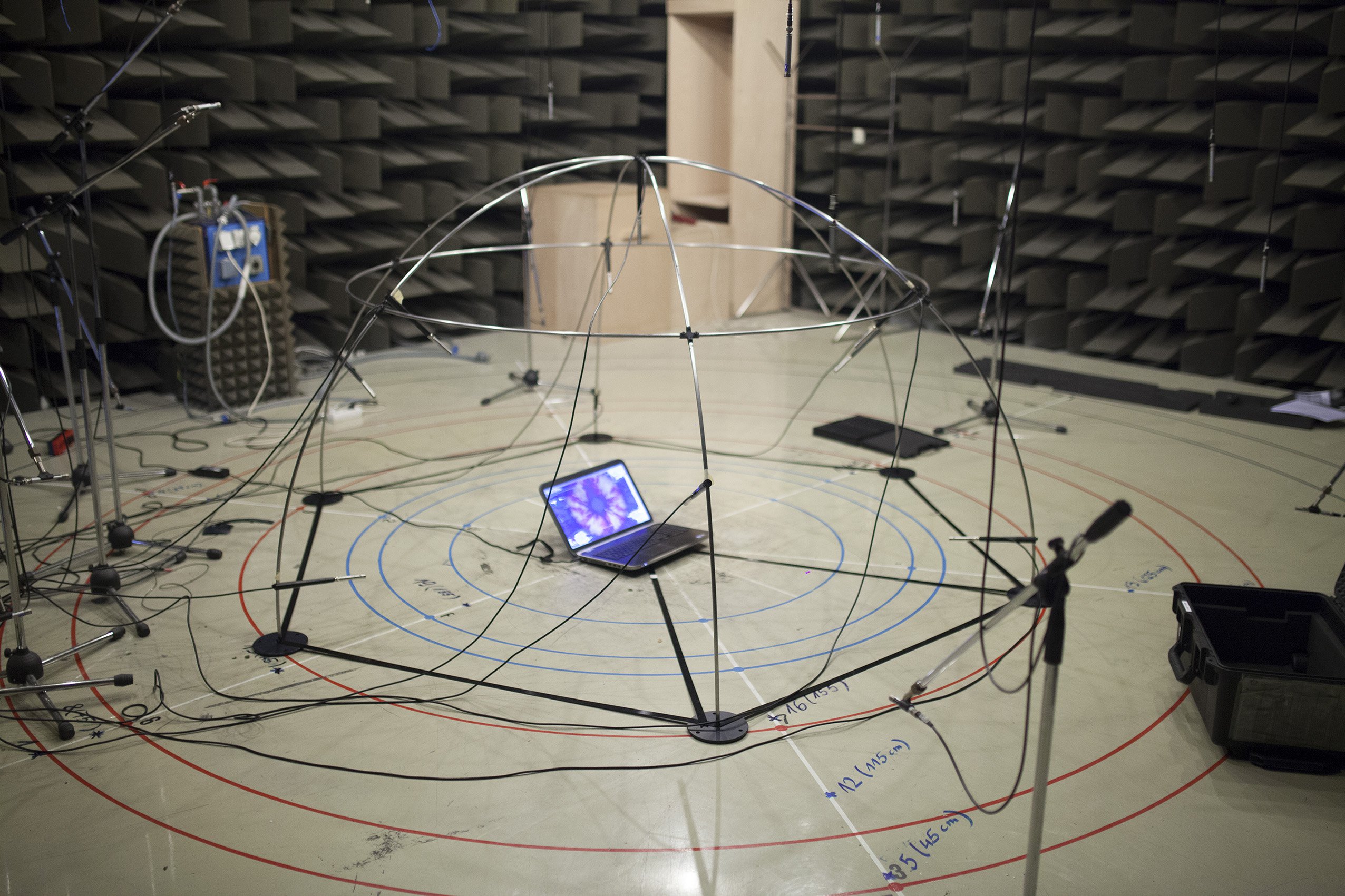
Image 2: Sound pressure level representation 

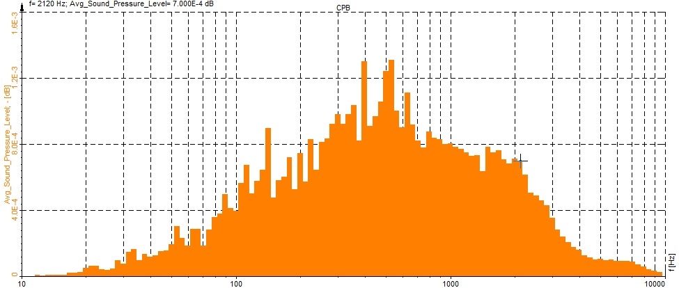
Ears detect the changes in sound pressure. Human hearing does not have a flat spectral sensitivity (frequency response relative to frequency versus amplitude). Humans do not perceive low and high frequency sounds as well as they perceive sounds near 2000 Hz, as shown in the equal-loudness contour. Because the frequency response of human hearing changes with amplitude, weighting curves have been established for measuring sound pressure.

The sound field is an area where the sound exists. When measuring the sound pressure, it is very important whether the sound field is free or diffused:

• Free sound field- it can be found in a space where there is no reflection. It can be simulated outside or in an isolation room, where all the sound that strikes the walls is absorbed. The main property of the free sound field is that the sound spreads spherically. 
  Image 3: Free sound field can be found in a space where there is no reflection

   

• Diffuse sound field- it can be found in a reverberation room. Sound reflects so many times, that it travels in all directions with the same probability. 
  Image 4: Diffuse sound field can be found in a reverberation room

   

Sound intensity

Sound intensity is defined as sound power per unit of an area. It depends on the distance from the sound source and the acoustic environment in which the sound source is. Sound intensity is a vector quantity and describes the amount and direction of the sound energy. The unit for sound intensity is [W/m²]. It is calculated as a product of the sound pressure and the speed of particles.

\( \overrightarrow{I} = p \overrightarrow{c} \)

Sound power

Sound power is the characteristic of a sound source, it is independent of the distance and, therefore, a practical way of comparing various sound sources. Sound power can be measured in different ways (by sound pressure or by sound intensity).

\( W = \int_{S}^{} I dS = \sum_{i=1}^{n} I_{i} S_{i} \)

Sound power level is determined by

\( L_{W} = 10log \left(\frac{W}{W_{0}}\right) \)

The SoundPower plugin performs the calculation by measuring the sound pressure.

Sound power is calculated by the following equation:

\( L_{W} = \overline{L_{P}} + 10 \cdot log_{10}\left(\frac{S}{S_{0}}\right) - K1 - K2 + C1 + C2 \)

• \( L_{W} \) = sound power
• \( L_{p} \) = sound pressure level
• \( S \) = measurement surface
• \( S_{0} \) = referenced surface (is by standard 1 m2)
• \( K_{1} \) = background noise correction
• \( K_{2} \) = room noise correction
• \( C_{1} \) = meteorological correction
• \( C_{2} \) = meteorological correction

For example, if we have a free-field measurement, and the microphones are aligned in a sphere, then L_p is the sound pressure level measured by 10 microphones, the surface S is 4πr², the background noise K₁ is the noise emitted from the machinery around the sphere, and there is no K₂ because we have free-field. C₁ and C₂ also stay zero, because the outside temperature is around 23°C and the altitude of the test site is below 500 meters sea level.

The Sound power plugin supports two standards for measuring sound power by measuring the sound pressure.

Both standards define:

• types of noise and noise sources,
• test environment,
• measurement uncertainty,
• criteria for background noise,
• criteria for air temperature and humidity,
• instrumentation equipment, and
• position of microphones.

Image 5: ISO standards 

ISO 3741 - specifies precision methods for determining the sound power level of a noise source from sound pressure levels measured in a reverberation test room (a room designed to create a  diffuse or random incidence sound field). The methods specified in ISO 3741 are suitable for all types of noise (steady, non-steady, fluctuating, isolated bursts of sound energy, etc.).

ISO 3744 - the standard specifies methods for determining the sound power level or sound energy level of a noise source from sound pressure levels measured on a surface enveloping the noise source (machinery or equipment) in an environment that approximates to an acoustic free field near one or more reflecting planes. The sound power level (or, in the case of noise bursts or transient noise emission, the sound energy level) produced by the noise source, in frequency bands or with A-weighting applied, is calculated using those measurements.

ISO 3745 - the standard specifies various methods for determining the sound power levels and sound energy levels of noise sources including machinery, equipment and their sub-assemblies. The selection of one of the methods from the series for use in a particular application depends on the purpose of the test to determine the sound power level or sound energy level and on the facilities available.

In order to facilitate the selection of the shape and dimensions of the measurement surface, the reference box shall first be delineated - clearly described. The reference box is a hypothetical surface defined by the smallest right parallelepiped that just encloses the source under test. When defining the dimensions of the reference box, elements protruding from the source which are known not to be significant radiators of sound may be disregarded.

The locations of the reference box, the measurement surface, and the microphone positions for measurements, are defined with respect to a coordinate system with origin O in the ground plane, shown in the pictures below. The point O is the middle point of a box consisting of the reference box and its images in the adjoining reflecting plane(s). The horizontal axes x and y of the coordinate system also lie in the ground plane, parallel to the length and width of the reference box. The characteristic source dimension, d_O, used to determine the dimensions of the measurement surface, is shown in the pictures below for reference boxes on one, two and three reflecting planes.

Images below show different positions of a reference box near the acoustically reflecting planes.

• \( d_{0}  \) - characteristic source dimension
• \( I_{1}  \) - reference box width
• \(  I_{2} \) - reference box length
• \( I_{3} \) - reference box height
• \(  O \) - origin of sound

One Acoustically Reflecting Plane

Image 6: One acoustically reflecting plane

 

Characteristic source dimension, in this case:

$$d_{0}=\sqrt{\left(\frac{l_{1}}{2}\right)^{2}+\left(\frac{l_{2}}{2}\right)^{2}+\left(l_{3}\right)^{2}}$$

Two Acoustically Reflecting Planes

Image 7: Two acoustically reflecting planes 

Characteristic source dimension, in this case:

$$d_{0}=\sqrt{\left(l_{1}\right)^{2}+\left(\frac{l_{2}}{2}\right)^{2}+\left(l_{3}\right)^{2}}$$

Three Acoustically Reflecting Planes

Image 8: Three acoustically reflecting planes

Characteristic source dimension, in this case:

$$d_{0}=\sqrt{\left(l_{1}\right)^{2}+\left(l_{2}\right)^{2}+\left(l_{3}\right)^{2}}$$

To use the Sound power plugin please download it from our webpage here and select SoundPower.dll. Please copy the file SoundPower.dll into the Addons folder of your Dewesoft X installation (e.g. D:\Dewesoft7\Bin\X3\Addons\), then start Dewesoft X.

To enable the plugin, first we have to go to the Settings inside Dewesoft X software. Click on the Extensions section and add a new plugin by clicking on the plus button. Find the Sound power plugin as it is shown on the image 9, and enable it.

Image 9: Enable Sound Power plugin 

When this is done, we can see the Sound power plugin enabled in the Extensions tree list. Next time we go to the Channel setup, Sound power icon will be there. See image 10.

Image 10: Sound power is now located in a Channel setup

ISO 3741 specifies precision methods for determining the sound power level of a noise source from sound pressure levels measured in a reverberation test room (a room designed to create a diffuse or random incidence sound field).

The methods specified in ISO 3741 are suitable for all types of noise (steady, non-steady, fluctuating, isolated bursts of sound energy, etc.).

The sound power level produced by the noise source, in frequency bands of width one-third-octave, is calculated using those measurements, including corrections that allow differences between the meteorological conditions at the time and place of the test and those corresponding to a reference characteristic impedance.

Measurement and calculation procedures are given for both a direct method (the method using the equivalent sound absorption area of the reverberation test room) and a comparison method (the method using a reference sound source of known sound power level) of determining the sound power level.

ISO 3741 is applicable to noise sources with a volume not greater than 2 % of the volume of the reverberation test room.

Image 11: Display view of an ISO 3741 

Hemisphere

The sound source is placed in the middle of the hemisphere. 

• When the sound source is placed over one acoustically reflective plane, the measurement surface is expressed \( S=2\pi r^{2} \). Key microphone positions are marked with numbers 1-10, additional positions are marked with numbers 11-20.

Image 12: Sound source is placed over one acoustically reflective plane
 

• When the sound source is placed over two acoustically reflective planes, the measurement surface is expressed \( S=\pi r^{2} \). Key microphone positions are marked with numbers 2,3,6,7 and 9, additional positions are marked with numbers 11,14,15 and 18. 
  Image 13: Sound source is placed over two acoustically reflective planes
  
  
• When the sound source is placed over three acoustically reflective planes, the measurement surface is expressed \( S=\frac{\pi r^{2}}{2} \). Key microphone positions are marked with numbers 1,2,3, additional positions are marked with numbers 4,5 and 6.
  Image 14: Sound source is placed over three acoustically reflective planes 

Parallelepiped

Parallelepiped measurement surface must have the same orientation as the reference box. The distance between the reference box and the measurement surface must be at least 0.25 m and is marked with \( d \).

Length, width, and height of the reference parallelepiped are marked with \( l_{1} \), \( l_{2} \), and \( l_{3} \).

• When the sound source is placed over one acoustically reflective plane, the measurement surface is expressed as \( S=4\left(ab+bc+ac\right) \)
  Image 15: Sound source placed over one acoustically reflective plane 

\( a=0.5l_{1} + d \)
\( b=0.5l_{2} + d \)
\( c=l_{3} +d \)

• When the sound source is placed over two acoustically reflective planes, the measurement surface is expressed as \( S=2\left(2ab+bc+2ac\right) \).
  Image 16: Sound source placed over two acoustically reflective planes 

\( a=0.5l_2+0.5d \)
\( b=0.5l_1+d \)
\( c=l_3+d \)

• When the sound source is placed over three acoustically reflective planes, the measurement surface is expressed as \( S=2\left(2ac+cb+ac\right) \).
  Image 17: Sound source placed over three acoustically reflective planes 

\( a=0.5l_1+0.5d \)
\( b=0.5l_2+0.5d \)
\( c= l_3+d \)

The parallelepiped in ISO 3744 has besides walls and corners also defined other types/sizes (small, tall, long, medium, large).

These types/sizes have the same equation for measuring the surface. The only difference is the number of microphones. That means that you can choose Small type/size and measure Large type/size device but you need to enter the correct value for the Number of microphones of Large type/size.

Cylinder

The reference box must be in the center of the cylinder. Distance between the cylinder and the reference box are marked with \( d_1 \), \( d_2 \), and \( d_3 \). The radius of the cylinder is expressed:

\( R=\left(\frac{l_1}{2}\right)+d_1 = \left(\frac{l_2}{2}\right)+d_2 \)

Height of the cylinder is expressed:

\( h=l_3+d_3 \)

Distances \( d_1 \) and \( d_3 \) must be set according to the size of the sound source (at least 0.5 m). From \( d_1 \) and \( d_3 \), we calculate \( h \) and \( R \) and also \( d_2 \):

\( d_2=R-\left(\frac{l_2}{2}\right) \)

Image 18: Distances for cylinder must be set according to the size of the sound source 

The whole measurement surface \( S  \) is the sum of the surface of the upper circle \( ST \) and the surface of the layer of the cylinder \( SS \).

• When the sound source lays on one acoustically reflective surface, surface \( ST=\pi R^2 \) and surface \( SS=2\pi Rh \).
• When the sound source lays on two acoustically reflective surfaces, surface \( ST=\frac{\pi R^2}{2} \) and surface \( SS=\pi Rh \). 
  Image 19: Surface calculation for one and two acoustically reflective surfaces

   

• When the sound source lays on three acoustically reflective surfaces, surface \( ST=\frac{\pi R^2}{4} \) and surface \( SS=\frac{\pi Rh}{2} \). 
  Image 20: Measurement surface calculation for three acoustically reflective surfaces

Standard describes different microphone arrangements around a sound source.

• The hemispherical measurement surface shall be centred on a point on the floor of the test room vertically beneath the assumed acoustic centre of the noise source under test, either the actual acoustic centre if known or the geometric centre if the acoustic centre is unknown. The measurement radius, r, shall satisfy all of the following conditions:
  • a) \( r \geq 2d_0 \) or \( r\geq 3h_0\), whichever is the larger, where \(d_0\) is the characteristic dimension of the noise source under test, and \(h_0\) is the distance from the acoustic centre of the source to the floor;
  • b) \(r\geq \frac{\lambda}{4} \), where \(\lambda\) is the wavelength of sound at the lowest frequency of interest;
  • c) \( r\geq 1 m\). 
• The measurement surface shall be wholly contained within the region of the hemi-anechoic room which is qualified for measurements. For small, low-noise sources to be measured over a limited range of frequencies, the measurement radius may be less than 1 m, but not less than 0,5 m. However, conditions a) and b) are relevant and a radius less than 1 m could itself impose limits on the frequency range over which tests are performed.

Image 21: Microphone positions for the hemispherical measurement surface 

• The spherical measurement surface shall be centred on the acoustic centre of the noise source under test, either the actual acoustic centre if known or an assumed acoustic centre such as the geometric centre of the source. The measurement radius, r, shall satisfy all of the following conditions:
  • a) \(r\geq2d_0\), where \(d_0\) is the characteristic dimension of the noise source under test;
  • b) \(r\geq\frac{\lambda}{4}\), where \(\lambda\) is the wavelength of sound at the lowest frequency of interest;
  • c) \(r\geq1 m\).
• The measurement surface shall be wholly contained within the region of the anechoic room which is qualified for measurements. For small, low-noise sources to be measured over a limited range of frequencies, the measurement radius may be less than 1 m, but not less than 0,5 m. However, conditions a) and b) are relevant and a radius less than 1 m could itself impose limits on the frequency range over which tests are performed. The area of a spherical measurement surface is \( S = 4 \pi r^2\).

Image 22: Microphone positions for the spherical measurement surface 

In order to take a scientific measurement with a microphone, its precise sensitivity must be known (in volts per pascal - V/Pa). Since this may change over the lifetime of the device, it is necessary to regularly calibrate measurement microphones.

Microphones can be calibrated in two ways. First, we have to know that the direct value of measurement from the microphone is the sound pressure in Pa. Therefore, we need to scale it to the physical quantity.

Scaling with a Calibration Certificate

If we don't use the calibrator but have the sensitivity of microphones, we can define it directly in the Channel setup.

Image 23: Calibration Chart  

First, Pa is defined as the physical unit of measurement. Next, we go to Scaling by function, check the Sensitivity, and enter the value in mV/Pa, which can be found on the calibration certificate of the microphone.

Image 24: Setting up the microphone scaling 

Calibrating the Microphone with the Calibrator

Another way is to calibrate the microphone with the calibrator. In this case, the known parameter is the sound level emitted by the calibrator. In our case, it is 94 dB (at 1000 Hz).

Image 25: Calibrating the microphone with the calibrator 

First we have to enter the channel setup of the microphone. The sensitivity is set to 1 by default. On the right side of the microphone scaling section, we can see information from the microphone, which is placed in the calibrator. Calibration frequency is set to 1000 Hz and the current value detected by the microphone is 127.4 dB. This is, of course, wrong because our calibrator has an output value of 94 dB. After we press Calibrate, the microphone's sensitivity will be measured from the highest peak in the frequency spectrum, usually at 1000 Hz (using of course amplitude correction to get right amplitude). Microphone sensitivity can be also read from TEDS. In that case, there is no need for calibration, because sensitivity is written on TEDS.

After we press the Calibrate button, we can see that the sensitivity has changed. Also, under the current value we can see the number 94 dB. This means that our microphone is now calibrated.

Image 26: With a click on the Calibrate button the Sensitivity scaling will change 

A human ear doesn't have an equal "gain" at different frequencies. We will perceive the same level of sound pressure at 1 kHz louder than at 100 Hz. To compensate for this "error", we use frequency weighting curves, which give the same response as the human ear has. The most commonly known example is frequency weighting in sound level measurement where a specific set of weighting curves known as A, B, C, and D weighting as defined in IEC 61672 are used. Unweighed measurements of sound pressure do not correspond to perceived loudness because the human ear is less sensitive at too low and high frequencies. The curves are applied to the measured sound level, by the use of a weighting filter in a sound level meter.

Image 27: Frequency weighting curves

As opposed to the FFT analysis, which has a specific number of lines per linear frequency (x-axis), CPB (constant percentage bandwidth, called also octave) has a specific number of lines if a logarithmic frequency x-axis is used. Therefore, the lower frequencies have a higher number of lines and the higher frequencies have a lower number of lines. CPB analysis is traditionally used in sound and vibration field.

CPB filter is a filter whose bandwidth is a fixed percentage of the centre frequency. The width of the individual filters is defined relative to their position in the range of interest. The higher the centre frequency of the filter, the wider the bandwidth. The bandwidth is defined in octaves or as a fixed percentage of the centre frequency of the filter.

Filters which all have the same constant percentage bandwidth (CPB filters) e.g.1/1 octave, are normally displayed on a logarithmic frequency scale. Sometimes these filters are also called relative bandwidth filters. Analysis with CPB filters (and logarithmic scales) is almost always used in connection with acoustic measurements, because it gives a fairly close approximation to how the human ear responds.

The widest octave filter used has a bandwidth of 1 octave. However, many subdivisions into smaller bandwidths are often used. The filters are often labelled as “Constant Percentage Bandwidth” filters. A 1/1 octave filter has a bandwidth of close to 70% of its centre frequency. The most popular filters are perhaps those with 1/3 octave bandwidths. One advantage is that this bandwidth at frequencies above 500 Hz corresponds well to the frequency selectivity of the human auditory system. Filter bandwidths down to 1/96 octave have been realised.

A detailed signal with many frequency components shows up with a filter shape as the dotted curve when subjected to an octave analysis. The solid curve shows the increased resolution with more details when a 1/3 octave analysis is used.

1/1 Octave filter

 

Image 28: 1/1 octave filter 

1/3 Octave filter

 

Image 29: 1/3 octave filter 

1/12 Octave filter:

 

Image 30: 1/12 octave filter 

The Dewesoft X3 Sound Power module can be split into the following sections:

Image 31: Sound Power setup 

Basic section

Under the Basic section, we have to choose the standard, according to which we are measuring. Depending on which standard we have chosen, we can select different microphone positions.

Image 32: Select appropriate measuring standard

ISO 3741

For direct and comparison method, the minimum distance between the noise source and the nearest microphone position is defined with the volume of the reverberation room \( V \), reverberation time \( T_{60} \) and a constant \( D_1\), where:

• \(D_1=0.08 \), and
• \( D_1=0.16\) for the frequencies below 5000Hz.

\(   d_{min} = D_1 \sqrt{\frac{V}{T_{60}}}   \)

ISO 3744/639x

There are few Microphone positions between which you can choose from:

• Parallepepid,
• Cylindric,
• Hemisphere, and
• Custom
  
  

Also, the Device type/size needs to be defined then:

ISO 3745

With ISO 3745 the Microphone positions can be defined as Hemisphere, Sphere, or Custom.

ISO 3743

ISO 3743 specifies methods for determining the sound power level or sound energy level of a noise source by comparing measured sound pressure levels emitted by this source (machinery or equipment) mounted in a hard-walled test room, the characteristics of which are specified, with those from a calibrated reference sound source.

User entered coordinates for microphone position section 

Image 33: Enter microphone coordinates option 

If we check the Enter mic. coordinates checkbox, we can define microphone positions ourselves. We have to define X, Y, and Z coordinates of each position.

Geometry section

In order to calculate the sound power, we need the surface of the reference box (device). Depending on the microphone positions the parameters change.

	Parallelepiped	Sphere and Hemisphere	Cylinder
Description	L1, L2, L3 represent width, depth, height of the measuring device, and d, which is the distance between the device and measured surface.	Insert the radius of the measurement surface.	Insert values L1, L2, L3 which represents the width, depth, length of the measured device and D1, D2, D3, which are width, depth, and length distance between device and measurement surface.
Image preview	Image 34: Parallelepiped definition	Image 35: Sphere and hemisphere definition	Image 36: Cylinder definition

Surface correction factor

From geometry distances the software also calculates the surface correction factor Ls that is used in sound power calculation.

\( L_S=10log\left(\frac{S}{S_0}\right) \)

\(S\) is the measurement surface and \(S_0\) is the reference measurement surface, where \(S_0 = 1 m^2\).

ISO 3741, ISO 3744 and ISO 3745 also specify the number of microphones, depending on the chosen geometry setup. If the number of microphones differs from the standard, you will get a warning but you can continue.

Image 37: Standard related warning 

If you have fewer physical microphones than microphone locations, you can align them in groups and move through them step-by-step during measurement (e.g. rotate them through four positions in cylindrical arrangement). In the end, all data will be combined. As some standards require 20 microphones and more in order to lower the costs for equipment you can align e.g. 5 microphones in a group and then move them through all 4 positions step-by-step during measurement, after that all data is combined automatically.

Image 38: Defining the number of microphones and groups 

Microphone position

In the Microphone positions section you can assign the analog channels to the positions, just click on the text fields and select from the drop-down menu. The X, Y, Z coordinates of microphones, as well as the groups, are shown.

In case the number of microphones is bigger than the maximum in standard ISO 3741, ISO 3744, or ISO 3745, then the coordinates will become zero.

Image 39: Assigning the microphone channels to the positions 

If you check the Enter mic. coordinates checkbox, you can enter the coordinates of microphones manually.

In the analysis setup, we have to select CPB resolution as well as bandwidth, frequency weighting, and measurement time. It is also possible to change and recalculate these offline after the data file is stored.

Octave settings

For the frequency analysis, constant percentage bandwidth (CPB) is used. You can choose between 1/1 octave or 1/3 octave.

Image 40: Octave setting 

Filters that all have the same constant percentage bandwidth (CPB filters) e.g. 1/1 octave are normally displayed on a logarithmic frequency scale. Sometimes these filters are also called relative bandwidth filters. Analysis with CPB filters (and logarithmic scales) is almost always used in connection with acoustic measurements, because it gives a fairly close approximation to how the human ear responds.

The widest octave filter used has a bandwidth of 1 octave. However, many subdivisions into smaller bandwidths are often used. The filters are often labeled as Constant Percentage Bandwidth filters. A 1/1 octave filter has a bandwidth of close to 70% of its center frequency. The most popular filters are perhaps those with 1/3 octave bandwidths. One advantage is that this bandwidth at frequencies above 500 Hz corresponds well to the frequency selectivity of the human auditory system.

Bandwidth

In the Bandwidth section, you can choose the frequency band for the calculation. Values are chosen from the drop-down menu. They depend on (and will change with) the selected acquisition rate and selected octave settings (1/1 or 1/3).

Image 41: Bandwidth selection 

Weighting

Because the human hearing is non-linear, it is required to apply frequency-weighting. The plugin supports type A-weighting and none weighting (linear). A-weighting is applied in an effort to account for the relative loudness perceived by the human ear.

Image 42: Apply frequency weighting 

Measurement conditions

Measurement time is an operational period or the operational cycle of the noise source under test for which the time-averaged sound pressure level is determined.

Measurement time affects the certainty of the measurement. The measurement time interval should be at least 20 seconds or longer.

Image 43: Measurement conditions definition 

In Offline calculation, we can place cursors (L1 and L2) and then chose the calculations between those two cursors. See image 43.

Repeatability

The uncertainty due to the repeatability of measurements of the sound pressure level is the closeness of agreement between results of successive measurements carried out under the same conditions;
it may be obtained from the standard deviation of repeatability using six measurements of the decibel sound pressure levels uncorrected for background noise at a single microphone position.

Measurement repeatability can be strongly influenced by averaging time. If the averaging time does not cover a sufficient number of machinery cycles, the total uncertainty may be unacceptably large for an engineering grade standard. For extremely low noise sources, reduction of background noise can reduce the sensitivity coefficient and hence total uncertainty by up to a factor of two.

Component of uncertainty could be lowered by better control of machinery operating conditions, use of longer averaging times, or by averaging multiple measurements made with appropriately modified conditions to represent a typical case.

Image 44: Repeatability definition 

History channels of multiple runs

Select the option Number of runs (e.g. operation modes of a sound source)if you want to measure sound power level and sound pressure level. See image 44.

Select the run during the measurement from the drop-down list.

Image 45: Select defined run 

In case you want to rename the runs, select the Runs editor button which is located right to the option Number of runs, and change the name of the run that it suits your application.

Image 46: Run settings

In the exported result matrix you will see the SPL of each microphone at each run and also the average values.

Image 47: Exported matrix results 

The sound power measurement can also be triggered with trigger channel (e.g. light barriers) instead of clicking the buttons for start and stop measurement.

Image 48: Enable trigger channels 

Select the Use trigger channels checkbox and select the first and the second trigger channels from the drop-down menu. Trigger channels can be synchronous, asynchronous, or single value channels.

For defining the trigger and retrigger level enter the settings for triggers.

Image 49: Trigger settings

One Trigger channel

The same channel can be used to start and stop the measurement.

Image 50: Using one trigger in both conditions 

Measurement is started by the first detected trigger edge on the trigger channel and is stopped by the trigger edge on the same trigger channel.

Image 51: Measurement is started by the first detected trigger edge on the trigger channel and is stopped by the trigger edge on the same trigger channel 

Different trigger channels

We can use one channel to start and the second channel to stop the measurement.

Image 52: Using different triggers 

Measurement is started by the first detected trigger edge on the first trigger channel and is stopped by the inverted trigger edge on the second trigger channel.

Image 53: Measurement is started by the first detected trigger edge on the first trigger channel and is stopped by the inverted trigger edge on the second trigger channel.

 

C1 and C2 meteorological corrections are used in the case that the air temperature at the test site is below 23°C or the altitude is higher than 500 meters above sea level. When you activate this option, it will be immediately calculated and written next to the label. You can either enter barometric pressure or altitude and the other value will be calculated automatically.

Image 54: C1 and C2 corrections are used in case of lower temperatures or higher altitudes 

 

C1 is the reference quantity correction, in decibels, to account for the different reference quantities used to calculate decibel sound pressure level and decibel sound power level, and is a function of the characteristic acoustic impedance of the air under the meteorological conditions at the time and place of the measurements:

Image 55: C1 calculates decibel sound pressure level and decibel sound power level 

C2 is the acoustic radiation impedance correction (in decibels), to change the actual sound power relevant for the meteorological conditions of the time and place of the measurement into the sound power under reference meteorological conditions. The value shall be obtained from the appropriate noise test code, but in the absence of a noise test code, the following equation is valid for a monopole source, and is a mean value for other sources:

Image 56: C2 changes the actual sound power into the sound power under reference meteorological conditions 

K1 background noise correction

K1 is by standard defined as the background noise correction. This is applied in different situations, please refer to the standard. K1 can be measured before switching on the sound source or afterward calculated by correctly placing the cursors on the measured data.

K1 correction is applied to the mean (energy average) of the time-averaged sound pressure levels over all the microphone positions on the measurement surface, to account for the influence of background noise.

Background noise correction is expressed in decibels [dB].

Image 57: K1 method option 

You can also define the K1 correction factor as a table. Measure the K1 once, and use the same correction multiple times. In K1 table editor enter the correction factors for each frequency band.

Image 58: Enter values option provides you the K1 editor 

K2 room correction

K2 corrects the influence of the room noise. K2 correction is applied to the mean (energy average) of the time-averaged sound pressure levels over all the microphone positions on the measurement surface, to account for the influence of reflected or absorbed sound. Environmental correction is expressed in decibels [dB].

Three methods are implemented in the Sound power plugin:

K2 room correction option	Description	Preview
Mean absorption grade	Please enter the room size and the mean absorption grade according to the standard.	Image 59: Mean absorption grade
Reverberation time	These parameters can be determined by acoustic measurement.	Image 60: Reverberation time
Enter values	An editor is provided, click first Create K2 table. Please ensure you have selected the correct bandwidth first, otherwise, the table will be reconfigured when changing bandwidth and values would get lost. The entered values in the table will be saved to the Dewesoft setup.	Image 61: Enter values
Calculate from RSS	Uses measured values from reference sound source with known sound power.	Image 62: Calculate from RSS

When you go to Measure mode, there is an auto-generated display called SoundPower. At first, all the graphs are empty.

Image 63: SoundPower display is auto-generated as you transit to Measure mode 

• Action buttons are provided on top to enable the user to go through the different steps of acquiring background noise and then start the real measurement, as well as switching between microphone groups.
• The Message, Status, and Warning displays show the progress (e.g. 17,2 / 20-sec done; K1 background acquiring...) and warnings if certain conditions are not fulfilled (e.g. Acquisition finished early....).
• On the left side, the input signals are shown: overall sound pressure levels of the microphones in the digital meters and CPB plots below.
• On the right side, the output signal show SoundPower and Overall Sound Pressure of all microphones in the digital meters, and the CPB plots of SoundPower, SoundLevel, and corrections.

For this example, 4 microphones are used and aligned in 2 groups, which means the setup has to be changed once in between. The measurement time stayed at 20 sec, which is the default value.

Image 64: Example microphones setup 

The flowchart for the following example is shown on image 65. With the previous and next buttons, you can switch between the groups and also repeat a measurement, as long as all the data for the group is not acquired.

Image 65: Example flowchart

Start storing (the sound source is switched off!); note that nothing will change on the display yet. Now click Acquire background (K1), wait for 20 sec; progress is shown in the status display.

Image 66: With click on Acquire background (K1) you activate the K1 background noise acquisition 

After K1 Acquisition is finished, switch on the sound source. Click Start Acquisition, wait again 20 sec. The four-microphone CPB plots (Group A) below should fill with data.

Image 67: Switch on the sound source, change from K1 to Run 1 and click on Start acquisition button 

Image 68: Group A is now filled with data 

After the acquisition is done, switch off the sound source. Change the microphone setup. The four microphones should move to their second position. Then change to Group B. 

Image 69: Change to group B 

Click Acquire background (K1) and wait 20 sec. Sound source must stay switched off. As the microphone positions changed, we have to repeat the K1 measurement for this position.

Image 70: Acquire background (K1) for the group B 

Now switch on the sound source again and choose Run 1 instead of K1 measurement. We click Start Acquisition and wait for 20 sec. After that, also the other four displays on the left side (Group B) should fill with data.

In the end, the text Sound power measurement finished should be shown. The display below gives more details if something went wrong (Warning). The CPB displays on the right side show SoundPower, SoundLevel, and K1 factor results.

Image 71: Sound power measurement results

The sound power plugin also supports offline calculation, which means changes in calculations can be done on the measured data (changing of the microphone groups, however, is not possible).

It's even possible to only collect raw data at the test site and perform all calculations afterward in the office. Therefore, one should be sure to have enough data, for the standard 20-second noise and 20 seconds with the sound source switched on. Below you see an example with the minimum data (here with 3 microphones):

Image 72: Collecting raw data for the standard 20-second noise and 20 seconds with the sound source switched on 

In the analysis mode, when the data file is open, go to Offline math and add the Sound power module. Do all the settings in the setup, ...

Image 73: In offline math add the Sound power module 

Then return to Review and click on Recalculate. Probably the calculation did not work yet, and you got a warning if you were using K1 correction. Please see the next page on how to place the cursors.

Image 74: Offline recalculation

We need to provide the plugin the information where the background noise is, and where to look for the sound source data. There are four different ways to place the cursors when performing an offline sound power analysis.

• If we perform the offline calculation without cursors placed and locked, the plugin will take 20 seconds of data from the beginning of the data file. This option will not consider the K1 correction factor.
  
  Image 75: Cursors are placed and locked
  
  
• If you only lock the first cursor at a fixed position, the plugin will take 20 seconds of data from the cursor position. This option will not consider the K1 correction factor.
  
  Image 76: The first cursor is locked at a fixed position
  
  
• With this option, we calculate the K1 background correction factor and the sound power level of the sound source. Lock the first cursor at the beginning of the background noise signal and lock the second cursor at the beginning of the part of the signal, where the sound source was turned on.
  
  Image 77: Lock the first cursor at the beginning of the background noise signal and lock the second cursor at the beginning of the part of the signal 
• lock the cursors and select Calculate between two cursors (L1 and L2).
  
  
  Image 78: Enable option 
  
  
  Image 79: Place cursors and recalculate the data between them 
  
  

To lock the cursors, first, place them at the desired position and then click on the cursor symbols to the left - the cursors are locked now.

Image 80: Lock the cursors 

The calculation is performed, when we press the Recalculate button.

HINT: You can also perform the calculation on only one specific part of the data. Use the recorder instrument and zoom into the interesting area.

Let's make an example with offline calculation. We have collected raw data from 4 microphones. For about 40 seconds, the sound source was OFF and then we switched it ON.

In the picture below we can see the data file, with raw data from microphones.

Image 81: Collected raw data from Mic 1 

First, we have to place the cursors, to tell the program, where the beginning of the noise and the beginning of the signal is. The first cursor represents the beginning of the noise, and the second cursor represents the beginning of the signal with the sound source turned on. After we have placed the cursors, we have to lock them.

Image 82: Place cursors and lock them 

The next step is to set up the SoundPower plugin. Go to Offline math and select Sound Power. Select the ISO standard, microphone position, and the number of microphones. Measurement time should be at least 20 seconds - it will take 20 seconds of data after our placed cursor.

Image 83: Set up the Sound Power Plugin

Then go back to Review and click the Recalculate button. After the recalculation is done, we can see that the sound power measurement is finished.

Image 84: After the recalculation is done, you will be able to see the complete result of the measurement

We measured the sound power level of a laptop in three different states and the minimum measurement time for one measurement is 20 seconds (according to standard).

We used the hemisphere kit from G.R.A.S with 10 microphones and a radius of 1.36 meters. The distance from the sound source to the microphones was 1 meter. The grid is very simple to assemble if you follow the attached instruction manual. It took us approximately 30 minutes to prepare everything. First, we had to put together the metal sticks and attached them together, to get a nice hemisphere structure. The next step was to put the microphones in the right positions according to the standards. The grid supports 10 or 20 microphones, so we had to select the right position for microphone mounting. The positions had to be the same as in standards and they are already predefined with small screws of different colors.

Image 85: Hemisphere kit of a radius 1.36m with a distance from the sound source to the microphones of 1 meter

We used 10 BNC cables that were 10 meters long, so that measurement equipment was outside of the semi-anechoic room. This is very important for reducing background noise to a minimum. Microphones had TEDS chip, and were calibrated in the factory. The whole data acquisition process took us approximately 10 minutes.

Image 86: Dewesoft hardware and software coupled together 

Setup was done like in the picture below.

Image 87: PID setup 

Image 89: Measurement screen

Results are shown as CPB analysis and with an overall dB number.

Image 90: Results are shown as CPB analysis and with an overall dB number 

When the calculations are finished, there are multiple options on how to export the data from Dewesoft X.

Image 91: Exporting the measurement data in different formats 

We can either print the current display arrangement or export to the clipboard or to external software.

For the first option just click on the button Print, and select the printer, which can also be a PDF writer.

Image 92: Printing the current display 

A quick way to export the data is by using the clipboard. Click on the instrument, e.g. the Octave plot showing the K1 correction data, to set it active. Then select Copy to clipboard -> Widget data from the Edit menu. Open MS Excel and paste the data into, the columns and rows will be filled exactly with the data you see.

Image 93: Copying data to clipboard
 

Or use the default export into a lot of different file formats, such as Matlab, Excel, Diadem, RPCIII, CSV, etc.. as it was shown on image 91.

After the sound power measurement has been done, you can easily export data into a prepared Excel template to automatically create your report by just pressing a button.

All the needed files for creating SoundPower report can be found on our website under the download section:

Image 94: Download the SoundPower report

Needed prerequisites:

• Microsoft Excel has to be installed
• Import the data header file SoundPowerDataHeader.xml in the Dewesoft X Settings - Data header. Then select when to ask the user to enter the details (Ask for header on start, Ask for header on end).
  
  Image 95: Import the data header file SoundPowerDataHeader.xml in Dewesoft X settings
• Copy the template files to your local Dewesoft X Script folder (e.g. D:\Dewesoft\System\X2\Scripts):
  • SoundPowerReport.xps
  • SoundPowerReport1.xlt
  • SoundPowerReport1.xltx

Creating the report

Restart Dewesoft X, open an existing sound power data file (the data header must have been filled during the measurement!), go to Export and select the Excel ribbon. The "Sound power" template should be visible now in the list on the left.

Then deselect all channels in the list on the right. Synchronous channels would take too much time to export and we don't need them for the report.

Image 96: Deselect all channels 

From the Sampling column select only the "Single value channels", which will include all CPS plots and final results.

Image 97: Select only single value channels

Then click Export. Excel will automatically start and fill all the data into the template.

Image 98: Data will be exported automatically

Notice that the Excel file contains multiple sheets:

• DataInfo - the data header details
• Events - events like start and stop storing, or notes added during measurement
• Single value - sound power CPB and overall levels
• Data1 - usually contains full-speed-data (e.g. with 50 kHz), but we deselected it
• Results - the final report

The blue marked sheets are automatically filled with data, the orange is just linked to them.

The result sheet is linked to other pages as it is shown on image 99.

Image 99: Result sheet is linked to the other pages

 

Modifying the template

If you want to change the example template (e.g. company logo, ...), select the Edit template.

Image 100: Edit template

Excel will open the template file (notice the ending .xltx).

Image 101: Template will be already filled out with the current data 

The template is already filled with the current data. To modify a cell, just press the equal sign (=), then you can move to one of the automatically filed sheets...

Image 102: Press the equal sign 

...select the wanted cell and press Enter.

Image 103: Select the wanted cell and press Enter 

The cell will be linked now.

Image 104: Cell will be linked now 

After you have done all your changes. it is important that you delete all the contents from all other pages except "RESULTS"!

Then press Save in Excel.