Sound pressure measurement

Sound is a wave motion in the air or in other elastic media. It is caused by the objects vibrating at specific frequencies (loudspeakers, reeds, machinery).

If an air particle is displaced from its original position, elastic forces of the air tend to restore it to its original position. Because of the inertia of the particle, it overshoots the resting position, bringing into play elastic forces in the opposite direction, and so on. Sound is readily conducted in gases, liquids, and solids such as air, water, steel, concrete, and so on, which are all elastic media.

Sound cannot propagate without a medium - it propagates through compressible media such as air, water, and solids as longitudinal waves and also as transverse waves in solids. The sound waves are generated by a sound source (vibrating diaphragm or a stereo speaker), which creates vibrations in the surrounding medium. As the source continues to vibrate the medium, the vibrations are propagating away from the source at the speed of sound and are forming the sound wave. At a fixed distance from the sound source, the pressure, velocity, and displacement of the medium vary in time.

Image 1: Propagation of a sound through media

 

Wavelength and frequency

In the picture below a sine wave is illustrated. The wavelength λ is the distance a wave travels in the time it takes to complete one cycle. A wavelength can be measured between successive peaks or between any two corresponding points on the cycle. This is also true for periodic waves other than the sine wave. The frequency f specifies the number of cycles per second, measured in hertz (Hz).

Image 2: Wavelength and frequency

 

Sound pressure

Sound pressure or acoustic pressure is the local pressure deviation from the ambient (average, or equilibrium) atmospheric pressure, caused by a sound wave. In the air, sound pressure can be measured using a microphone, and in water with a hydrophone. The SI unit for sound pressure p is the pascal (symbol: Pa).

Sound pressure level

Sound pressure level (SPL) or sound level is a logarithmic measure of the effective sound pressure of a sound relative to a reference value. It is measured in decibels (dB) above a standard reference level. The standard reference for the sound pressure in an air or other gases is 20 µPa, which is usually considered the threshold of human hearing (at 1 kHz). The following equation shows us how to calculate the Sound Pressure level (Lp) in decibels [dB] from sound pressure (p) in Pascal [Pa].

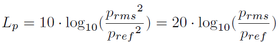
where pref is the reference sound pressure and pRMS is the RMS sound pressure being measured.

Most sound level measurements will be made relative to this level, meaning 1 pascal will equal an SPL of 94 dB. In other media, such as underwater, a reference level (pREF) of 1 µPa is used.

The minimum level of what the (healthy) human ear can hear is SPL of 0 dB, but the upper limit is not as clearly defined. While 1 bar (194 dB Peak or 191 dB SPL) is the largest pressure variation an undistorted sound wave can have in Earth's atmosphere, larger sound waves can be present in other atmospheres or other media such as underwater, or through the Earth.

Image 3: Sound pressure level of different real-life scenarios

 

Ears detect changes in sound pressure. Human hearing does not have a flat frequency response relative to frequency versus amplitude. Humans do not perceive low- and high-frequency sounds, as well as they, perceive sounds near 2000 Hz. Because the frequency response of human hearing changes with amplitude, weighting curves have been established for measuring sound pressure. We will learn in this course how to make a measurement and how to "distort" the results that they will match with what the human ear is "measuring".

A human ear doesn't have an equal "gain" at different frequencies. We will perceive the same level of sound pressure at 1 kHz louder than at 100 Hz. To compensate for this "error", we use frequency weighting curves, which give the same response as the human ear has. The most commonly known example is frequency weighting in sound level measurement where a specific set of weighting curves known as A, B, C and D weighting as defined in IEC 61672 are used. Unweighed measurements of sound pressure do not correspond to perceived loudness because the human ear is less sensitive at too low and high frequencies. The curves are applied to the measured sound level, by the use of a weighting filter in a sound level meter.

Image 4: Frequency weighting curves

 

• A-weighting: A-weighting is applied to measured sound levels in an effort to account for the relative loudness perceived by the human ear. The human ear is less sensitive to low and high audio frequencies.
• B-weighting: B-weighting is similar to A, except for the fact that low-frequency attenuation is less extreme (-10 dB at 60 Hz). This is the best weighting to use for musical listening purposes.
• C-weighting: C-weighting is similar to A and B as far as the high frequencies are concerned. In the low-frequency range, it hardly provides attenuation. This weighting is used for high-level noise.
• D-weighting: D-weighting was specifically designed for use when measuring high-level aircraft noise in accordance with the IEC 537 measurement standard. The large peak in the D-weighting curve reflects the fact that humans hear random noise differently from pure tones, an effect that is particularly pronounced around 6 kHz.
• Z-weighting (linear): Z-weighting is linear at all frequencies and it has the same effect on all measured values.

As opposed to the FFT analysis, which has a specific number of lines per linear frequency (x-axis), CPB (constant percentage bandwidth, called also an octave) has a specific number of lines if a logarithmic frequency x-axis is used. Therefore, lower frequencies have a higher number of lines, and higher frequencies have a lower number of lines. CPB analysis is traditionally used in the sound and vibration field.

CPB filter is a filter whose bandwidth is a fixed percentage of the center frequency. The width of the individual filters is defined relative to their position in the range of interest. The higher the center frequency of the filter, the wider the bandwidth. The bandwidth is defined in octaves or as a fixed percentage of the center frequency of the filter.

Filters, which all have the same constant percentage bandwidth (CPB filters) e.g.1/1 octave, are normally displayed on a logarithmic frequency scale. Sometimes these filters are also called relative bandwidth filters. Analysis with CPB filters (and logarithmic scales) is almost always used in connection with acoustic measurements because it gives a fairly close approximation to how the human ear responds.

The widest octave filter used has a bandwidth of 1 octave. However, many subdivisions into smaller bandwidths are often used. The filters are often labeled as Constant Percentage Bandwidth filters. A 1/1 octave filter has a bandwidth of close to 70% of its center frequency. The most popular filters are perhaps those with 1/3 octave bandwidths. One advantage is that this bandwidth at frequencies above 500 Hz corresponds well to the frequency selectivity of the human auditory system. Filter bandwidths down to 1/96 octave have been realized.

A detailed signal with many frequency components shows up with a filter shape as the dotted curve when subjected to an octave analysis. The solid curve shows the increased resolution with more details when a 1/3 octave analysis is used.

Example of a 1/1 octave filter:

Image 5: Example of a 1/1 octave filter

 

Example of a 1/3 octave filter:

Image 6: Example of a 1/3 octave filter

 

Example of a 1/12 octave filter:

Image 7: Example of a 1/12 octave filter

 

A microphone is an acoustic-to-electric transducer or a sensor that converts sound in the air into an electrical signal.

Microphones are basically pressure sensors, but they are dedicated to the measurement of very small variations of pressure around the atmospheric pressure.

All microphones convert sound energy into electrical energy, but there are many different ways of doing the job, using electrostatics, electromagnetism, piezo-electric effects, or even the change in resistance of carbon granules. The majority of microphones used in applications are either capacitor (electrostatic) or dynamic (electromagnetic) models. Both types employ a moving diaphragm to capture the sound, but they use a different electrical principle for converting the mechanical energy into an electrical signal. The efficiency of this conversion is very important because the amount of acoustic energy produced by voices and musical instruments is small.

Image 8: An example of a microphone

 

How does a microphone work?

Different types of microphones have different ways of converting sound energy, but they all share one thing in common: a diaphragm. This is a thin piece of material (such as paper, plastic, or aluminum) which vibrates when it is struck by sound waves. In a typical hand-held microphone, the diaphragm is located in the head of the microphone.

Image 9: Operation of a microphone explained

 

When the diaphragm vibrates, it causes other components in the microphone to vibrate. These vibrations are converted into an electrical current which becomes the audio signal.

The way in which a microphone transforms an input signal from the acoustic to the electrical signal is known as its transducer principle.

1. The condenser microphone is the most widely used type. It is based on the principle that the capacitance of two electrically charged plates will change with their separation distance - it transforms an acoustic signal into an electric one by using a capacitor. In microphones, this capacitor is formed by the backplate and the light diaphragm, which moves in response to acoustic pressure variations. The diaphragm of the microphone is actually used as one element of this capacitor; when the acoustical signal causes the diaphragm to move, the distance between it and the other half of the capacitor is affected, creating the electrical output signal A condenser microphone is essentially a capacitor, with one plate of the capacitor moving in response to sound waves. The movement changes the capacitance of the capacitor, and these changes are amplified to create a measurable signal. Condenser microphones usually need an external power supply or a small battery to provide a voltage across the capacitor. 
   Image 10: A condenser microphone

    

    A capacitor has two plates with a voltage between them. The diaphragm vibrates when struck by sound waves, changing the distance between the two plates and therefore changing the capacitance. Specifically, when the plates are closer together, capacitance increases and a charge current occurs. When the plates are further apart, capacitance decreases, and a discharge current occurs. Condenser microphones usually need a small battery or external power to provide a voltage across the capacitor.
2. 
   
3. A dynamic microphone takes advantage of the electromagnetic effects. When a magnet moves past a wire (or coil of wire), the magnet induces an electrical current to flow in the wire. In a dynamic microphone, the diaphragm moves either a magnet or a coil when the sound waves hit the diaphragm, and the movement creates a small current. Using this electromagnet principle, the dynamic microphone uses a wire coil and magnet to create the audio signal. 
   Image 11: A dynamic microphone

    

4. Piezoelectric microphone - piezoelectric microphones feature sensitive crystals that respond to the physical vibration of the acoustic signal coming into the microphone and create the electrical output. While this technology was once widely used in tape recorders, it is most commonly used today in pickup devices for acoustic instruments. 
   Image 12: Piezoelectric microphone

    

5. Loudspeakers perform the opposite function of microphones by converting electrical energy into sound waves. This is demonstrated perfectly in the dynamic microphone which is basically a loudspeaker in reverse. 
   Image 13: Loudspeaker

    

6.  

A microphone's directionality or the polar pattern indicates how sensitive it is to sound arriving at different angles about its central axis. The pattern of microphones describes a three-dimensional orientation in space relative to sound sources in the ambient environment. Microphones can be divided into omnidirectional and unidirectional devices.

• Omnidirectional microphone (non-directional microphone) can absorb acoustic signals from any input direction.
• The unidirectional microphone can use several different polar patterns or shapes that indicate from which direction they will best receive an acoustic signal.

The unidirectional audio pattern is great for focusing on a specific sound and blocking out ambient noise. Unidirectional microphones are highly directional and must be pointed directly at the subject to capture the best sound quality.	Image 14: Unidirectional microphone
Cardioid microphones are unidirectional microphones that absorb an acoustical signal in a heart-shaped pattern. This sound pattern makes these microphones good vocal microphones, as they can absorb the dynamic range of a vocal performance while not capturing signals from other directions.	Image 15: Cardioid microphone
The omnidirectional microphone is gathering a wide range of sounds from all directions. This kind of microphone is most accurate at the representation of the total environment. It collects sound equally well from all directions.	Image 16: Omnidirectional microphone
Bidirectional microphones receive a balanced signal from both the front and back of the microphonic element and are the best to use when we must capture the interplay of two sound sources.	Image 17: Bidirectional microphone

Selecting a microphone involves a number of choices:

• externally polarized or pre-polarized,
• free-field, pressure or random incidence,
• dynamic range,
• frequency range.

Externally polarized or pre-polarized

Condenser type microphones require a polarization voltage that can either be supplied from an external power supply or the microphone itself can be polarized by injecting a permanent electrical charge into a thin PTFE layer on the microphone backplate.

Externally polarized microphones

These microphones are used with standard preamplifiers. The preamplifier must be connected to a power module or an analyzer input which can supply the preamplifier with power as well as 200 V for polarization. Externally polarized microphones are the most accurate and stable and are preferred for very critical measurements.

Pre-polarized microphones

These microphones are used typically with constant current power preamplifiers. Pre-polarized microphones must be connected to an input stage for constant current power transducers or be powered by a constant current power supply.

Constant current power preamplifiers use standard coaxial cables. The long-term stability and high-temperature stability of pre-polarized microphones are not as good as for externally polarized microphones.

Free-field, pressure or random incidence

Measurement microphones can be divided into three groups: free-field, pressure, and random incidence. The differences between microphones from group to group are at the higher frequencies, where the size of a microphone becomes comparable with the wavelengths of the sound being measured.

Free-field microphones

A free-field microphone is designed essentially to measure the sound pressure as it was before the microphone was introduced into the sound field. At higher frequencies, the presence of the microphone itself in the sound field will disturb the sound pressure locally. The frequency response of a free field microphone has been carefully adjusted to compensate for the disturbances to the local sound field.

Image 18: Free-field microphone

 

Free-field microphones are recommended for most sound pressure level measurements for example with sound level meters and sound power measurements.

Pressure microphones

A pressure microphone is for measuring the actual sound pressure on the surface of the microphone's diaphragm. A typical application is in the measurement of sound pressure in a closed coupler or, as shown below, the measurement of sound pressure at a boundary or wall; in which case the microphone forms part of the wall and measures the sound pressure on the wall itself.

Pressure microphones are recommended for studies of sound pressures inside closed cavities.

Image 19: Pressure microphone

 

Random incidence microphones

A random incidence microphone is for measuring in sound fields, where the sound comes from many directions e.g. when measuring in a reverberation chamber or in other highly reflecting surroundings. The combined influence of sound waves coming from all directions depends on how these sound waves are distributed over the various directions. For measurement microphones, a standard distribution has been defined based on statistical considerations; resulting in a standardized random incidence microphone.

Random incidence is used typically for sound pressure level measurements according to ANSI standards.

Image 20: Random incidence microphone

 

The dynamic range of a microphone

The dynamic range of a microphone can be defined as the range between the lowest level and the highest level that the microphone can handle. This is not only a function of the microphone alone but also of the preamplifier used with the microphone. The dynamic range of a microphone is, to a large extent, directly linked to its sensitivity.

In general, a microphone with high sensitivity will be able to measure very low levels, but not very high levels, and a microphone with low sensitivity will be able to measure very high levels, but not very low levels. The sensitivity of a microphone is determined by the size of the microphone and the tension of its diaphragm. A large microphone, with a loose diaphragm, will have a high sensitivity and a small microphone, with a stiff diaphragm, will have low sensitivity.

The upper limit of the dynamic range

The highest levels that can be measured are limited by the amount of movement allowed for the diaphragm before it comes into contact with the microphone's back plate.

As the level of the sound pressure on a microphone increases, the deflection of the diaphragm will accordingly be greater and greater until, at some point, the diaphragm strikes the back plate inside the body of the microphone. This is ultimately at the highest level the microphone can measure.

The lower limit of the dynamic range

The thermal agitation of air molecules is sufficient for a microphone to generate a tiny output signal, even in absolutely quiet conditions. This thermal noise normally lies at around 5 V and will be superimposed on any acoustically excited signal detected by the microphone. Because of this, no acoustically excited signal below the level of the thermal noise can be measured.

The frequency range of a microphone

The frequency range of a microphone is defined as the interval between its upper limiting frequency and its lower limiting frequency. With today's microphones, it is possible to cover a frequency range starting from around 1Hz and reaching up to 140 kHz.

Low-frequency measurements require a microphone with a well-controlled static pressure equalization with a very slow venting. Special versions are available for infrasound measurements.

High-frequency measurements are very sensitive to diaphragm stiffness, damping, and mass, as well as diffraction.

Upper limiting frequency

The upper limiting frequency is linked to the size of the microphone, or more precisely, the size of the microphone compared with the wavelength of sound. Since wavelength is inversely proportional to frequency, it gets progressively shorter at higher frequencies. Hence, the smaller the diameter of the microphone, the higher are the frequencies it can measure. On the other hand, the sensitivity of a microphone is also related to its size which also affects its dynamic range.

Lower limiting frequency

The lower limiting frequency of a microphone is determined by its static pressure equalization system. Basically, a microphone measures the difference between its internal pressure and the ambient pressure. If the microphone was completely airtight, changes in barometric pressure and altitude would result in a static deflection of its diaphragm and, consequently, in a change of frequency response and sensitivity. To avoid this, the microphone is manufactured with a static pressure equalization channel for equalizing the internal pressure with ambient pressure. On the other hand, equalization must be slow enough to avoid affecting the measurement of dynamic signals.

We can connect the condenser microphone directly to the ACC or the ACC+ module. We used a pre-polarized free-field microphone which already has an integrated preamplifier.

Image 21: Condenser microphone connected to SIRIUS DAQ device

 

A condenser microphone needs a power supply. When we select the IEPE mode, the excitation for the microphone will be provided. We can choose between 4 and 8 mA excitation.

Image 22: Channel setup of a microphone in Dewesoft 

 

In order to take a scientific measurement with a microphone, its precise sensitivity must be known (in volts per pascal - V/Pa). Since this may change over the lifetime of the device, it is necessary to regularly calibrate measurement microphones.

Microphones can be calibrated in two ways. First, we have to know that the direct value of measurement from the microphone is the sound pressure in Pa. Therefore, we need to scale it to the physical quantity.

Scaling with a calibration certificate

If we don't use the calibrator but have the sensitivity of microphones, we can define it directly in the Channel setup.

Image 23: Calibration certificate of a microphone

 

First, Pa is defined as the physical unit of measurement. Next, we go to Scaling by function, check the Sensitivity, and enter the value in mV/Pa, which can be found on the calibration certificate of the microphone.

Image 24: Entering the sensitivity value from the calibration certificate

 

Calibrating the microphone with calibrator

Another way to calibrate the microphone is with the calibrator. In this case, the known parameter is the sound level emitted by the calibrator. In our case, it is 94 dB (at 1000 Hz).

Image 25: Sound calibrator

 

First, we have to enter the channel setup of the microphone. The sensitivity is set to 1 by default. On the right side of the microphone scaling section, we can see information from the microphone, which is plugged in the calibrator. The calibration frequency is set to 1000 Hz and the current value detected by the microphone is 127.4 dB. This is, of course, wrong because our calibrator has an output value of 94 dB. After we press Calibrate, the sensitivity of the microphone will be measured from the highest peak in the frequency spectrum, usually at 1000 Hz (using of course amplitude correction to get the right amplitude). Microphone sensitivity can be also read from TEDS. In that case, there is no need for calibration, because sensitivity is written on TEDS.

Image 26: Signal from a microphone, before the calibration

 

After we press the Calibrate button, we can see that the sensitivity has changed. Also, under the current value, we can see the number 94 dB. This means that our microphone is now calibrated.

Image 27: Signal from a microphone, after the calibration

 

The Sound level Math section allows calculation of the typical parameters for sound level measurements from a single microphone. It allows for Dewesoft to be used as the typical sound level meter. With appropriate hardware (Sirius ACC) it can easily fulfill all the requirements for a Class I sound level meter. It supports also different standards: IEC60651, IEC60804, IEC61672.

Sound level measurements are available selecting the Sound level meter checkbox under Math section.

Image 28: Adding new Sound Level Meter module

 

After selecting this option, a tab labeled Sound levels appears in the Dewesoft Setup screen.

Basic procedures of Sound level measurement are:

• channel setup
• microphone calibration
• measurement

This value is calculated directly in the Medium & Calibration field of the sound level module channel setup. We connect the calibrator to the microphone and turn it on. We can see the signal directly in the small overview. In our case, it should be a sine wave with a frequency of 1000 Hz. Since all the frequency weighted curves are referenced to 1000 Hz, this is a very usual frequency for calibrating microphones.

We can also choose the medium in which we are measuring. It can be chosen from Air or Water, the difference is in reference sound pressure.

Image 29: Calibration of a microphone in the Sound Level Meter module

 

After we see that the sound is correctly recognized as the sine wave at 1000 Hz, we can click the Calibrate button to perform a calibration. The sound module will calculate the Sensitivity of a microphone from the highest FFT amplitude and reference value.

Image 30: Calculated sensitivity of a microphone

 

The sensitivity will already be directly corrected in the source channel and, therefore, no additional analog scaling is necessary. We can directly check the calibrated sensitivity of the information found on the calibration certificate.

Now we have to check if the calibration was successful. Set a sampling rate of at least 5 kS/s - we would recommend 20 - 50 kS/s - and enter the FFT analysis. Set the FFT options to Flat top filter and the Y scale type to dB Noise. Now press the RMS icon to display the RMS values within the FFT graph. Switch on again your microphone calibrator and the RMS values should display 94 dB.

Image 31: FFT spectrum of a microphone with calibrator ON

 

If there are mismatches you should do the calibration again.

Because of differences in their construction, microphones have their own characteristic responses to sound. This difference in response produces non-uniform phase and frequency responses.

The dynamic range of a microphone is the difference in SPL (sound pressure level) between the noise floor and the maximum sound pressure level. The sensitivity of a microphone indicates how well the microphone converts acoustic pressure to output a voltage (unit: mV/Pa). A high sensitivity microphone creates more voltage and vice versa.

Microphones are not uniformly sensitive to sound pressure and can accept differing levels without distorting. For scientific applications, microphones with a more uniform response are desirable, but this is often not the case for music recording, as the non-uniform response of a microphone can produce a desirable coloration of the sound. This is why the comparison of published data from different manufacturers is difficult because different measurement techniques are used.

The frequency response diagram plots the microphone sensitivity in decibels over a range of frequencies (typically 20 Hz to 20 kHz). The frequency response may be stated as: "30 Hz - 16 kHz ±3 dB". This is interpreted as meaning a nearly flat, linear, plot between the stated frequencies, with variations in amplitude no more than plus or minus 3 dB. Commonly made statements such as "20 Hz - 20 kHz" are meaningless without a decibel measure of tolerance. Directional microphones frequency response varies mostly with distance from the sound source, and with the geometry of the sound source.

The noise level is the sound pressure level that creates the same output voltage as the microphone does in the absence of sound. This represents the lowest point of the microphone's dynamic range (it is important if you wish to record quiet sounds). The measure is often stated in dB(A), which is the equivalent loudness of the noise on a decibel scale, frequency-weighted for how the ear hears (A-weighting).

Example 1

In the example below, we measured the sound that comes from an accordion. The condenser microphone was placed near the accordion and we measured the beating frequency of the signal. The signal from the microphone clearly shows that the accordion has more than one clean tone. We hear two closely spaced frequencies as a beating.

Image 32: Time-domain signal of an accordion

 

Example 2

The next example with the condenser microphone was made with a cantilever beam. We measured the beams natural frequency. The microphone was plugged in ACC module and it was set to IEPE mode. It was calibrated as it was described on the previous pages. We excite the beam with a hammer and then it vibrates with its own frequency.

Image 33: Measurement of tuning fork vibrations with microphone

 

The signal from the microphone was put into the FFT analyzer.

Image 34: FFT spectrum of a tuning fork 

 

The first peak in the FFT spectrum of the signal from the microphone was at 91.55 Hz. That was also very close to the beam's natural frequency measured with the frequency response function math (91 Hz).