Statistical Calculations on Sampled Data

Dewesoft has many different data acquisition sources. Taking raw data measurement is often not enough to come to the wanted result, so data processing is one of the most important features that allows you to recalculate signals, filter them or make any other signal processing.

1. The following section will give you an overview of the statistics and counting math module and show you how to use it for different purposes.

Enabling Mathematics

Statistics module is located inside mathematics module, so first you have to make sure that the mathematics module is enabled. On the Dewesoft Setup screen, next to the Analog and the other available tabs, a Math tab has to be displayed as shown on the picture below.

Image 1: Enabling Math module in Dewesoft X

You can add a new statistic in Dewesoft Math -> Add math,  where we can choose between three types of statistics:

• Basic statistics,
• Array statistics and
• Classification.

Equally Counting can be found and added in Add math drop-down window.

Image 2: Statistics and Counting can be find in Add math drop-down window

We add a new Basic statistic with adding it under Add math, as it was described before or we can adjust the existing ones with click on the Setup button on  the upper right corner of already activated Basic statistics line. In both cases following will open:

Image 3: Basic statistics setup window

According to the picture above, in general we can divide Basic statistics setup window in four major parts:

Output channels - Statistical functions

To select statistical function simply click (check) on the box beside its name on Output channels section:

Image 4: Calculation Output channel options

• RMS will calculate the root mean square value of the signal.
• Quadratic RMS is similar to the RMS, except all the values are double squared and summed.
• Median is the numerical value separating the higher half of a data sample from the lower half. 
• Average will calculate the average or middle point.
• Peak is the maximum deviation of the signal from the average value.
• Peak-peak is the difference between the minimum and maximum.
• Crest factor is the ratio between the peak and RMS value. Crest factor gives an impression about the spikes in the signal. Pure sine waves have a crest factor of 1.41.
• Sum provides the sum of all acquired values in respect of the selected calculation type (sample or time dependent).
• Minimum will calculate a minimum value of the signal for the specified period.
• Maximum will calculate a maximum value of the signal for the specified period. This is very intensive operation and therefore unavailable in Running mode.
• Time of minimum calculates exact time of minimum value.
• Time of maximum calculates exact time of maximum value.
• Variance is indicating how possible values of a signal are spread around the expected value.
• COV (coefficient of variation) is normalized measure of dispersion of probability distribution. It is calculated as ration between standard deviation and the mean.
• Standard deviation is a measure of the spread of the values of the signal away from its mean, measuring how widely spread the values in a data set is. If the data points are close to the mean, then the standard deviation is small (if all the data values are equal, then the standard deviation is zero).

Calculation type

In this section five basic calculation types will be described: 

• Block based,
• Running,
• Single value,
• Triggered blocks and
• Start-stop blocks.

Time and Sample based calculation

Before we jump into calculation types we need to mention that Block based and Running calculation type are calculated according to the specified Time interval or numbers of Samples.

Image 5: Time based and Sample based options for calculation

• Time based (in seconds) defines the time interval for calculation. 0,1 second in our case means that it will calculate the statistical quantities in 0,1 second interval. Therefore the resulting channels will have an update interval of 0,1 second. 
  With time based calculation each signal is recalculated to a synchronous sample and then each of those synchronous samples is used as an input element for statistics calculation.

• Sample based (number of samples) defines number of samples used for calculation, so resulting channels will have an update interval of defined sample block size. It is important to know that every single sample is used as an input value for statistics calculation.

Asynchronous signals are not interpolated, in fact their each value is deployed to the next sample.

Examples: 

• Single value, Sample based calculation: 
  If you have only two samples in a measurement and their values are 5 and 10, the Single value average for a Sample based calculation will equal 7.5 and it is calculated independently of time or when those two samples were acquired.
  
  
• Single value, Time based calculation:
  In this case the calculation is based on time, so the average can be anywhere between 0 and 10. Average now depends of each sample's time duration and it takes into account when the signals were acquired. So if we have in 10 seconds long measurement two samples acquired, where one sample has a value of 5 at 2 seconds and the other has a value of 10 at 4 second as it is shown on the Image 6, the Single value average will equal to 7.

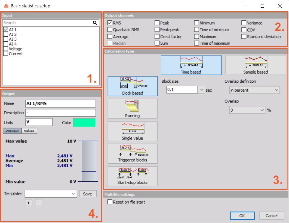
Image 6: Single value average of a time based calculation explanation

Block based

Block based calculation calculates the statistical quantity based on a specific time interval defined by the block size.

Image 7: Block based calculation type window

• Block size you can define by time or sample.

• Overlap is useful when we need a specific time interval, but still want to have a higher update rate of the resulting channels. Overlap defines (same for as FFT averaging) how much 'old' data is taken into account for the next calculation. This increases the result update rate with the same number of lines. It can be defined in percent or as absolute value.
  
                                                                                              Image 8: Overlap definition window

In this case on the picture, the quantities will be updated in 0,1 second interval with 50% overlap. It means that the second block will not be calculated at the end of the first block, but half of the block before that. So the first block will be calculated from 0 to 0,1 second, second one from 0,05 to 0,15 second, third one from 0,1 to 0,2 second and so on.

Running

Running calculation is an extreme version of overlapping. The second block is calculated after one sample after the first block. Block size has the same meaning as for block based calculation.

Image 9: Running calculation type window

With this method, we can only calculate RMS, Average, Quadratic RMS, Variance and Standard deviation statistical functions, because all others would be too intensive (especially minimum and maximum while all others relate to those two).

Single value

Single value is the simplest calculation and has no settings. It will output only one value at the end of the measurement. The result will be updated also during the measurement, but only the final value will be stored in the data file.

                                                                                                Image 10: Single value calculation type window

Triggered blocks

Triggered blocks option calculates the statistical value based on a specific trigger event. The calculation begins at the start of the acquisition. When a trigger event is recognized, it stops the first calculation, writes the statistical value with its timestamp and then starts to calculate a new value. We can define any channel as the trigger channel and the settings for the trigger condition are the same as the alarm or storage triggers.

Image 11: Triggered blocks calculation type window

Start/Stop blocks

Start/stop blocks option calculates the statistical value starting at a specific trigger event. When an event is recognized, it starts to calculate. When a stop condition is recognized, then the value is written to the resulting channel with the timestamp of the stop event. It will wait with the calculation until the new start event is recognized. The start and stop channel can be any channel, also a different one and the trigger condition have the same options as the alarm or storage triggers.

Image 12: Start-stop blocks calculation type window 

With the array statistics, there are several options that can be chosen:

Image 13: Array statistics setup window

• Minimum finds minimum value from the array. There are two output channels created: class and value. Class will describe which index of the array holds the parameter and the value will be the minimum value itself.
• Index of minimum shows the position of minimum in array.
• Axis position of minimum shows the position of minimum in axis units.
• Maximum finds maximum value from the array. There are two output channels created: class and value. Class will describe which index of the array holds the parameter and the value will be the maximum value itself.
• Index of maximum shows the position of maximum in array.
• Axis position of maximum shows the position of maximum in axis units.
• Average calculates average value of all elements from the array.
• Sum calculates sum of all elements from the array.
• Variance calculates the variance of all elements from the array.

Array area

We can calculate Output channel from the full array area or we can specify custom array area.

Image 14: Array area definition

If we want to use only selected area from array of data we have to define the area (from, to). In those two boxes we have to define two numbers, which represents the coordinates of the array. The first number is the x-coordinate (0,0) and the second number is the y-coordinate (0,0).
While talking about arrays this would mean defining the top left corner and the bottom right corner of the table we want to use as an array area.

Classification in the measurement field is used for various applications, for example to find the distribution of power grid frequencies with the time or to find the distribution of sound levels to which certain area or working place is exposed to.

Default setup of classification math module looks like this:

Image 15: Classification setup window

Calculation type

Image 16: Calculation type window for Classification

First we need to define what will be the result of classification. This is done in calculation type area of classification setup and there are three options between which we can choose:

• Single value based - the result will be one array holding the result of the entire run.
• Block based -  the result will be a set of arrays, where each one will be added at the end of defined block size. Block size is defined in seconds, so If we have for example block size of 2 seconds and acquire data for 10 seconds, we will get 5 arrays of classification values, where each will be represent 2 seconds of data.
• Running - a running total is the summation of a sequence of numbers, which is updated each time a new number is added to the sequence, by adding the value of the new number to the previous running total.

Option Show class as a separate channel is only available when Single value based calculation type is selected. It will create a single value channel for each of the class element. This is a nice way to display the values in the multi meter.

Class definition

Image 17: Class definition for Classification

For class definition we have to set the:

• Lower limit sets the lower limit for the start of counting - all values below this level will be counted in the first class.
• Upper limit sets the upper limit for the end of counting - all values above this level will be counted in the last class.
• Class count defines the number of classes. In the example above the width of each class will be 5/20=0,25. The first and the last class will have half width, so it will go from from 0 to 0.125. Second class has a middle value of 0.25 and it goes from 0.125 to 0.375 and so on.

Histogram type defines what will be the output of the data (amplitude):

Image 18: Histogram types

• Absolute count - each class value has the number of samples within the class (value will always count up).
• Relative count - each class value has the value of samples with the class normalized to total number of counted samples (sum of all classes will be always 1).
• Relative count [%] - is the same as relative count, but expressed in percent (sum of all classes will be always 100).
• Density - provides empirical probability density, where each class value has the number of samples normalized to total number of samples and divided by class width. In this case the value is not depending on number of classes within a range.
• Density [%] - is the same as density, but multiplied with 100.
• Distribution -  provides empirical probability distribution, where each class value has the sum of all lower classes and the number of current samples, normalized to total number of samples. The highest class has the value of 1.
• Distribution [%] - is the same as distribution, but expressed in percent. The highest class has the value of 100.

Statistics and Distribution

Image 19: Statistics and Distribution windows

There are also several special output channels available, that are defined under Statisctics:

• Skewness is the asymmetry of probability distribution.
• Kurtosis represents the measure of "peakness" of distribution.

Additionally we can output a list of Distribution point values. Distribution points are the class values at which distribution reaches entered value.

For the moment the distribution points work only if distribution is chosen as the histogram type. Histograms can be seen in the 2D graph during the measurement and analysis. If we choose block based calculation, we can use also 3D graph to display the history of classifications.

Image 20: Histogram shown on 2D graph

Counting is the standard procedure to reduce amount of data for analysis. For example counting is used in applications of road load data collection where we have some static load and on top also a dynamic load.

As described in introduction section counting can be, the same as the statistics, found inside Dewesoft Math module and its default setup looks like this:

Image 21: Counting setup window

Counting is made based on rain-flow analysis. The reason for this is that the only interesting values for analysis are the height of load cycles and the average static load of that cycle. 

Counting setup definition

The counting procedures counts the peaks and the valleys of the signal.

Image 22: Counting setup definition

Local extreme detection

The Hysteresis under Local extreme detection is defined in percentage of class width. This prevents too many false counts if the signal is noisy.

Image 23: Local extreme detection

Algorithm settings

Image 24: Algorithm settings

There are several Counting Methods to choose from:

• Peak counting- counts the number of peaks in the signal in certain classes, where you can choose its counting direction:
  • peaks, 
  • valleys or 
  • both - peaks and valleys.
• Range counting -counts the range between successive peaks and valley pairs. Ranges are positive when slope between peaks and valleys is positive. We can choose either to count in:
  • positive, 
  • negative directions or
  • both directions.
• Level crossing - counts the number of times when that signal crosses various levels. Also as with range counting you have to choose counting direction.

Also there are three possible output values - Data normalization:

• Absolute - outputs number of the cycles as a value, where values will increase with time.
• Relative - it outputs the number of cycles normalized to absolute number of cycles - sum of all values will be always 1.
• Relative [%] - it outputs the number of cycles normalized to absolute number of cycles multiplied with 100 - sum of all values will be always 100.

Visualization

For all options we have to define also Visualization - the number of classes for the average value, minimum and the maximum value or we choose to define minimum and maximum value from the range of input parameters.

Image 25: Visualization setup