AC and DC Voltage Measurement

Electricity is very hard to imagine because we can not see if a voltage is present or if a current is flowing. If we want water to flow out of a pipe we need some water pressure which is achieved with a water pump. In electricity, our flow is the current, water pressure is the voltage and the pump is the battery. This means that the voltage is the cause of the current.

Voltage, sometimes also called electromotive force, is what makes electric charges move. It is an electrical potential difference between two poles, the positive and the negative.

The relationship between voltage, current, and resistance in a circuit.

Voltage can be either AC or DC, depending on the current that is carrying it. In DC systems, the current never changes direction. It is unidirectional, i.e., it does not change polarity.But in AC systems, the current alternates directions, crossing 0V in a positive direction, then turning around and crossing 0V again in a negative direction. You can see both DC and AC voltage (and current) represented in the graphs below:

DC circuits (left) versus AC circuits (right)

Electricity is very hard to imagine because we cannot physically see if the voltage is present or if a current is flowing, so we'll use a water analogy to try and explain how electrical circuits function. Water systems are simple to understand because we can physically see the water and the behavior that it possesses.


Image 1: High voltage sign

 Now let's take a look at how a water system behaves. It is a well-known physical fact that if the water is to flow out of a pipe the water needs to be pressurized, this is mostly achieved by a pump. In electricity, the flow is the current, water pressure is the voltage and the pump is the battery. This means that the voltage instigates the flow of the current like the water pressure is the cause of the volume flow rate of water.

The measurement device used for measuring voltage is called a voltmeter. Voltage is also known as the potential difference between two points, so the voltmeter is always connected in parallel to the circuit (see image 2). To influence the circuit as little as possible, the input impedance of the voltmeter has to be very high. The typical input impedance of the Voltmeter is 10 MOhm.

Image 2: Schematic illustration for connecting a voltmeter

Measuring voltage is the most basic measurement with Data Acquisition (DAQ) devices because most of the Analog-to-Digital converters (ADC) use voltage as the input value. That's why measuring voltage with DAQ seems simple, right? The answer is yes if we are measuring voltages in the range that is directly supported by the ADC. But when measuring very small voltages in the range of micro Volts (µV) or very high voltages up to several kilo-Volts (kV), an amplifier is needed to prepare the signal for the AD conversion. For both challenges Dewesoft has the right solution.

On the one hand the Low Voltage amplifier (LV and HS-LV) in combination with the 24-bit ADC technology allow for measurements of very low voltages even at high measurement ranges (e.g. µV resolution at a range of ± 10V).

On the other hand, the High Voltage amplifier (HV and HS-HV) allows the direct measurement of voltages up to 1600V DC (1200V DC at HS-module). For measuring voltages higher than 1600 VDC, voltage probes/dividers or voltage transducers can be connected to the instrument.

Isolation Voltage

When measuring voltage, it's important to choose the right amplifier range. Using the incorrect amplifier range can destroy the amplifier if the measured voltage exceeds the isolation voltage of the integrated amplifiers in the measurement instruments.

For example, measuring the public grid voltage (230 Vrms / 325 Vpeak) with a STG module can destroy the entire module as the isolation voltage is rated at 200 Vpeak for the measurement range below 10V and 300V peak for the measurement range above 10V. In order to measure voltages higher than ±100 V the use of the HV-amplifiers is mandatory.

Measurement Range

The appropriate selection of the measurement range is essential for high accuracy and reliable measurement results. There are a number of measurement ranges available with every amplifier which can be configured in the Dewesoft X channel setup. If the measurement range is too low, the signal will exceed the input range and errors and channel overloads will appear instead of correct values. On the other hand, if the measurement range is too high, the inaccuracy will be too high to make correct measurements.

The most precise measurement is achieved when the measurement value range coincides with the DAQ amplifier input range. In this case the highest resolution of the measurement is received with the same number of bits used by the AD converter.

Let's take a look at an easy example measuring voltage. If only one-tenth of the AD converter input range is used, the resolution of the outcome will only be one tenth of the actual performance of the AD converter. A 16-bit converter can read 65536 different discrete values, but the measurement will only consist of 6500 different values which is a very low resolution. Measuring a signal from 0 - 7 V will be pointless with a 1200V range (resolution 18 mV) instead a module with a 10V range should be used (resolution 0,15 mV) which will yield a much higher measurement resolution. That's why there are diverse modules with different input and measurement ranges available.

There is a variety of different voltage types, therefore the type of voltage needs to be identified. Voltage types include peak, peak-to-peak, average, RMS, AC and DC. The differences can be better explained using the image below.  

Image 3: Voltage types


The average voltage is, as the name already states, the average value for a certain time period. For pure sinusoidal signals (AC), the average will be zero.

The RMS voltage is the root-mean-square voltage and it is the square root of the arithmetic mean of the squared function values that define the continuous wave forms. It is the most commonly used value to define the AC voltage at a certain point and produces the same energy as the DC voltage at an ohmic load.

\( U_{RMS}=\sqrt{\frac{\sum_{n=0}^{N-1} u^2 (n)}{N}} \)

The peak voltage describes the highest voltage at any given period. In the datasheet specifications the peak voltage or the DC voltage of an input is given which means the same. To calculate the RMS value for sine waves, the peak value has to be divided by the square root of 2.

The peak-to-peak ratio shows the amplitude of positive and negative peaks in a period.

The Crest factor is the peak amplitude divided by the RMS value of the waveform.

\( C=\frac{\mid x\mid_{peak}}{x_{RMS}} \)

The rectified mean is the average of the rectified signal. In terms of an AC signal it's the average of the absolute value of voltage or current.

\(U_{RECT}=\frac{1}{T} \int\limits_{t=0} ^T \mid u \mid (t)  dt   \) 


Image 4: Voltage rectified mean

 The rectified mean is used e.g. for transformer testing as the rectified mean is proportional to the magnetic flux.


Basically, there are three different "types" of DAQ amplifiers: Single ended, differential and isolated amplifiers. These will be shortly explained below.

Single-ended

Single ended amplifiers have only one input pin because the second input pin is connected directly to the ground. Because of this kind of connection this amplifier is only suitable for measuring floating voltage sources where one output point can be connected to ground. This type of amplifier is easy to use but has two major disadvantages:

  • Unwanted ground loops
  • The amplifier is not isolated
Image 5: Schematic illustration of a single ended amplifier


A ground loop is an unwanted current from the sensor ground to the instrument ground because of a small difference in the ground potentials. These potential differences are in the micro volt (µV) region, but it can cause a large amount of noise in a measured signal.

An example of the problems that noise in a measurement can cause: a sensor with an output range of 10 V is connected to a single-ended amplifier, it is assumed that a dynamic range of 140 dB is needed. After a simple calculation, it is determined that the allowed potential difference between the sensor and the instrument ground is 1 µV. The solution for the potential difference is isolation of the sensor or the instrument.

Differential amplifier

The differential amplifier has two inputs separated from ground. This type of amplifier is the most common and amplifies the voltage difference between both inputs. With this technology it is possible to avoid ground loops but be careful of the common-mode input voltage.

Image 6: Schematic illustration of a differential amplifier

What is common-mode input voltage? One way to describe input common mode voltage (VICM) is that it is seen as the average voltage of the inverting and non-inverting input pins.

\( V_{ICM}=\frac{V_{in+}+V_{in-}}{2} \)

Another way to imagine a VICM: It is the voltage level common to both inputs Vin(+) and Vin(-). That means that the differential inputs of DAQ which measure the differences between inputs, the differentially measured value is the small, but common mode input voltage and can still be in hundreds of volts (current measurement with shunts).

Another term which describes differential amplifier inputs is input common-mode voltage range (VICMR). This is the parameter most often used in datasheets and is also the one that should receive the most attention. VICMR defines a range of common-mode input voltages in which the amplifier will work properly and describes how close the inputs can get to either supply rail. This means the potential of the input pins must be between supply voltages (V+ and V-).

Isolated amplifier

Using isolated amplifiers eliminates the disadvantage of single-ended amplifiers and differential amplifiers. They are independent of ground loops, common mode voltage, short circuits etc. These modules are isolated from the housing and the main board of the measurement device. Therefore, the amplifier will only "see" the difference of the absolute voltage. The high isolation voltage (compared to measurement range) allows safe and reliable operation also at voltage peaks, faults etc. and so enables the usage for an array of different applications.

After a short description of amplifiers, it can be said that the main advantage of differential amplifiers is the lower price. They are perfect for measurements with isolated sensors like strain gages or current clamps. Differential amplifiers also provide the high-quality measurement for non-isolated sensors, but engineers also need to know sensor behavior like common mode range or isolation to provide correct measurements. On the other hand, isolated signal conditions are more expensive, but a worry-free solution up to isolation voltage.

Let's take a look at how a low voltage measurement of up to 50V can be done. Voltages of up to 50V can be connected directly to a couple of different Dewesoft amplifiers. The amplifiers differ from each other in measurement range, isolation, bandwidth, noise, and extended functionalities.

Every measurement channel supports a number of input voltage ranges. The most precise measurement will be achieved when the input voltage range of the measurement channel is set in such a way that it coincides with the voltage of the measured signal.

The table below shows which Dewesoft amplifiers can be used for the measurement of voltages of up to 50V. The table also contains information about the maximal sampling rate and the bandwidth as well as the available measurement ranges for each amplifier.

Table 1: Dewesoft amplifies that can be used for voltage measurement up to 50 V

The common low-voltage amplifiers allow a sampling rate of up to 200 kS/s per channel with a maximal bandwidth of 75 kHz. The high-speed series (HS) is used for applications that require a high sampling rate and high bandwidths like voltage or current measurement in inverters. The sampling rate of the HS series is 1 MS/s. After choosing the right amplifier, the signal only needs to be connected to the amplifier.


Measuring voltages higher than 100 V require the use of the Sirius HV or HS-HV module. The Sirius HV module allows measuring voltages of up to 1200 VDC while the HS-HV module allows measuring voltages of up to 1600 VDC.

The table below shows the two different amplifiers for measuring high voltages with information about the measurement range, sampling rate, bandwidth and isolation.

Table 2: Dewesoft amplifiers that can be used for high voltage measurements up to 1600 V

Just as with low-voltage amplifiers the HS-series is designed for measuring very fast signals like Pulse-width modulation (PWM) regulated voltages of an inverter. Inverters operate at a switching frequency of up to 200 kHz which requires high bandwidth of the whole measurement chain and a high sampling rate. To allow analysis of every kind of application the maximal sampling rate of the HS-HV module is 1 MS/s.

HV vs. HS-HV

To simplify the choice of which one of the modules will fit better to which application, both modules will be used to measure the voltage of a PWM regulated 3-phase servo motor. The results will then be compared. Both of the module sample rates are set to the maximum, which is 200 kS/s for the HV module and 1 MS/s for the HS-HV module. Coarsely measured data will have some similarities, whereas the real difference will become apparent when the data of the PWM modulated sine wave voltages is further analyzed.

The first difference seen here is for the "chopped" sine. With an HV module (200kS/s) we get an overshoot when the signal "jumps". In the image below the measured motor voltage with the HV module with 200kS/s rate is depicted. The overshoot is clearly seen as little tick at start and stop of the voltage level shift.

When the signal is zoomed into for a better view of the resolution of the single samples, it becomes apparent that the reason for this overshoot is that the sample rate is too low. This happens because of the short rise time of the voltage therefore, there is only one or even no samples on the slope, which causes an error of measurement on the edges of our signal.

Image 7: Overshoot of samples which is caused by setting the sample rate too low

The HS-HV module has a higher bandwidth and therefore delivers 5 times more samples for the same measured time period, this means that there is no overshoot on the same measured signal. The cleaner transition is the result of more than one sample on the slope, this delivers a better resolution at the edges of the signal jump.

The problem with the overshoot begins at switching frequencies at around 2 kHz. At higher switching frequencies, it is expected that there will be even more differences between the dual core and the HS modules. To illustrate this a second measurement was done again using the voltage output of the frequency converter, but the frequency was increased to 16 kHz.


 The HS module can measure a much wider bandwidth than its dual-core counterpartImage 8: High speed amplifier vs. dual core amplifier bandwidth range

 The first obvious difference is seen in the bandwidth of the measured signal. With the dual core channel (blue) the frequency starts to damp at 66 kHz and there are absolutely no frequencies above 100 kHz in the measured signal. With the HS module (green) the dampening of the frequencies starts much later than that of the dual core. As seen in the image below the HS module can measure a much wider bandwidth than its dual core counterpart.

When observing both measured signals on the scope we see that the HS module is a few microseconds faster than the Dual core module.


The HS module is a few microseconds faster than the Dual-core moduleImage 9: High speed amplifier vs. dual core amplifier measurement speed

 Another difference that must be considered when measuring high-frequency voltages are the transients in the signal. The HS module is much better at transient measuring and yields a much better oscillation coverage after every peak.

Image 10: High speed amplifier vs. dual core amplifier transient recording


While voltage measurements up to 1 kV are relatively simple, things tend to get more complicated when measuring voltages over 1600 VDC because voltage probes/dividers or voltage transducers are necessary which adjust and reduce the voltage to a level that is suitable for the amplifier.

Image 11: High voltage warning


Voltages Probes (Voltage Dividers)

There are two different types of voltage probes: The pure resistor voltage probe (for AC and DC measurement) and the resistor-capacitive voltage probe (for AC measurement only). The input impedance of the voltage probe should be as high as possible; therefore, the input resistance should be as high as possible and the input capacitance as low as possible.

There are active, passive and differential voltage probes available.

Passive voltage probes: are simple, cheap and robust but have a high input capacitance and problems measuring low voltages.


Image 12: Schematic illustration of a passive voltage probe

Active voltage probes: have a high input resistance and low input capacitance but need an external power supply. They are a lot more sensitive and more expensive than passive ones.


Image 13: Schematic illustration of a active voltage probe

Differential Voltage Probes: Passive and active voltage probes are single-ended amplifiers with reference to earth. If a differential signal needs to be measured a differential voltage probe must be used.


Image 14: Schematic illustration of a differential voltage probe

The function of the voltage probe can be easily explained using a simple resistor voltage probe with the serial connection of two resistors with high resistance.

Image 15: Simple resistor voltage probe with the serial connection of two resistors 

When using a voltage divider with the same resistance value (R1 = R2), the voltage drop on one resistor will be half of the connected voltage. So, when measuring high voltages in the range of up to 2000 V, this simple transducer reduces the voltage to 1000 V. This is low enough to measure it using a Sirius high voltage module with an input range up to 1200 V.

Resistors with too low impedance, compared to a circuit in which voltage is measured will cause a substantial current spike. This current affects the measured circuit and reduces the accuracy of the measurement. The input impedance of the measurement instrument must be 100 to 1000 times higher than the value of R1, otherwise, the ratio will change, and the impedance of the measurement instrument must also be taken into account. Another factor that must be considered is the short circuit resistance which is the sum of R1 and R2 -> if this value is too low it will cause a short circuit.

When using a voltage probe, the ratio between the input and the output voltage must be calculated and adapted to the in-channel setup in the software. This ratio is important because the measured voltage of the measurement device must be multiplied by this ratio to yield the real voltage (Vin in the image).

\( V_{out}=\frac{V_{in}}{K_r} \)

\(  R_{1}=R_{2}=R \)

\( R_{S}=R_{1}+R_2=2R \)

\( K_{r}=\frac{R_{S}}{R_1} = \frac{2R}{R}=2 \)


Voltages Transducers

Voltage transducers are mainly used to monitor the voltage on the public grid. A voltage transducer is easily explained as a transformer in a no-load operation. On the input (primary) side, a high voltage signal is connected. On the output side of the voltage transducer, we get a low voltage signal which is directly proportional to the input voltage. In public grid operation the secondary voltage is standardized with a level of 100V respective 100V/sqrt(3). The level of 100 V/sqrt(3) is used in unipolar isolated voltage transducers in star connection. The level of 100 V is used in bipolar isolated transducers (line-line voltage).

There are different measurement classes of voltage transducers which describe the accuracy and phase shift of the transducers. The classes span from 0.1 to 3. Class 0.1 means that the accuracy of the measured amplitude is 0.1% and the phase shift is ± 5 minutes. At class 3 the accuracy is 3% and the phase shift ± 120 minutes.

Image 16: Schematic illustration of the working principle of a voltage transducer 
\( \frac{u_p}{u_s}\approx\frac{N_p}{N_s} \)


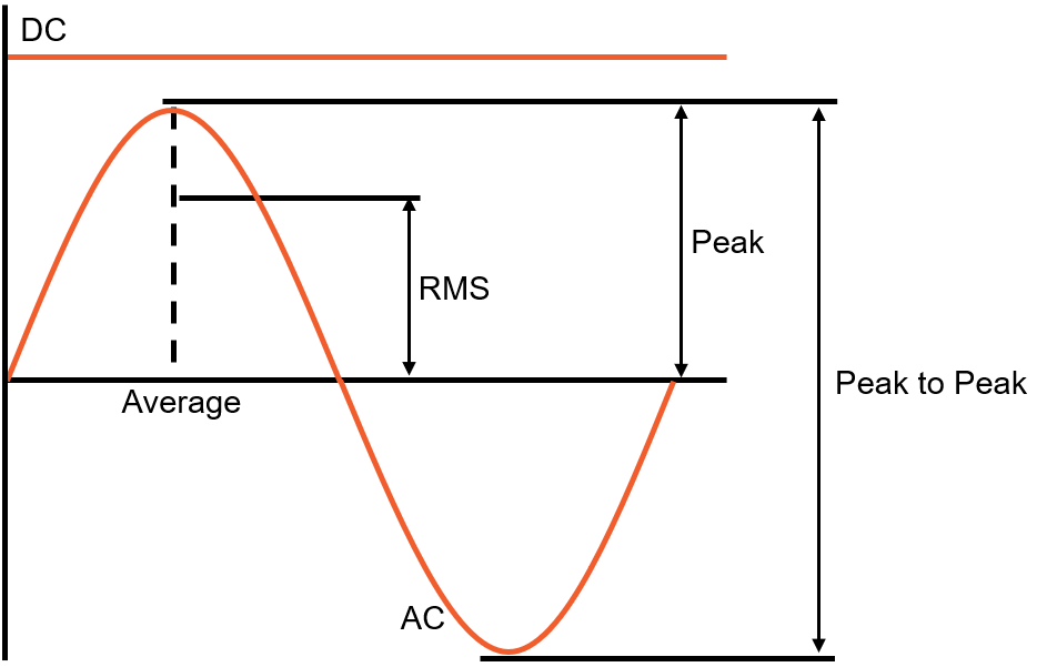
Following the theory, a practical example of how the Dewesoft measurement instruments work will follow. The voltage of the public grid will be measured. The value input voltage of the public grid must be considered to identify what type of amplifier input is needed for the measurement. The public grid in Europe is declared with a value of 230 VRMS but to ensure safe operation of the measurement instruments the peak values of the grid must be considered for the input range. The peak value of the grid in Europe equals the RMS value multiplied by the square root of 2 as seen in the equation below.

\( 230V_{RMS}\cdot\sqrt{2}\approx325V_{peak} \)

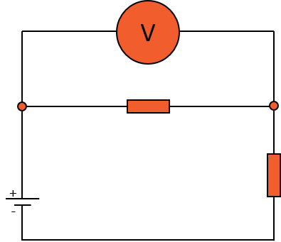
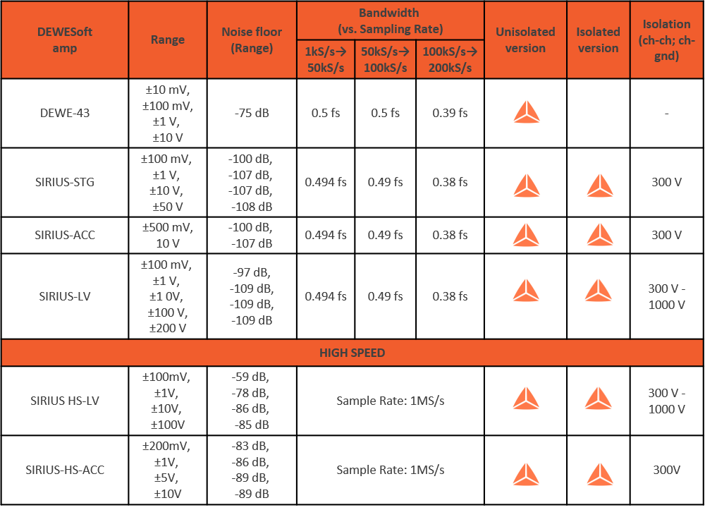
With a peak value of 325 V, we can directly use a Sirius HV-HS module that supports voltage up to 1.6 kV. This means that we can make a simple measurement without any additional voltage dividers or amplifiers and a simple connection as illustrated below. Channel 4 will be used, which has a Sirius HV-HS amplifier integrated into it. The other channels can be left inactive (unused in the software) as they are not relevant to this measurement. The next step is to configure the measurement channel setup in the software as illustrated below.

Image 17: Single-phase voltage connection to a Sirius 4xHV 4xLV

 There are two sides for the set-up window, the left side is the amplifier side and the right side is the sensor side.

Setting up the Physical quantityImage 18: Channel set up a screen in Dewesoft X

On the Amplifier side, we can toggle between the 50 V and 1600 V range. In this example, the 1600 V range will be used. A Low-pass filter can also be used to cut off the higher frequencies, but caution should be taken when doing that. If a frequency lower than half of the sample rate is taken it will cut the signal in the measurement range, this might be useful in some applications but mostly this configuration is set by mistake.

The setup on the Sensor side is about selecting which sensor is used for measurement. In this case, the voltage is directly measured without a sensor, so only the physical quantity must be set as Voltage and the unit as Volt (V). In this part of the setup, the scaling factor can also be set if sensors or dividers are used for the measurement. In this case, it will have the value 1 as the voltage is measured directly and no scaling is done.

For this example, the settings are done so the measurement can be started. By clicking on the Measure button. The best way to observe a sinusoidal waveform is with the scope. When the scope is first opened there will be a running wave that is impossible to analyze, this is due to the fact that the software is running in free mode, and the measurement needs to be held somehow. It is recommended to add a trigger on the norm trigger and defining the source and the trigger level. For the purposes of this example, it can be left as it is, as the trigger source is the U1 channel and the level equals 0.

Image 19: Measurement screen of voltage with a simple trigger 

DualCoreADC Mode

In the previous section a lot was said about proper amplifier measurement range selection. Now it's time to take a look at the impressive options offered by the dual core mode in the Sirius amplifiers. When using the Sirius dual-core mode it is possible to get a better resolution (less noise) at low amplitudes. That is solved with two 24-bit AD converters with different ranges on each channel.

The first AD converter has a full input channel range and the range of the second AD converter is only 5% of the full channel range. This technology measures the signal with low and a high gain simultaneously which means that the signal can be measured with a relatively high amplitude but at the same time it has a perfect resolution at low amplitudes of the same signal.

Let's take a look at the difference between dual core mode and normal mode when measuring low signals with a high range:

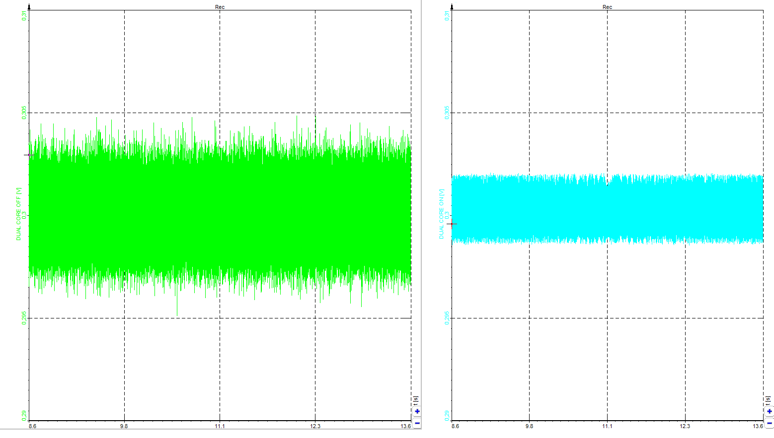
Image 20: Enabling the dual core mode in Dewesoft X

In this example a 0.3 V DC signal from the calibrator on two ACC amplifiers will be measured. On both amplifiers, a 10 V range will be chosen (which is complete nonsense) but it's the easiest way to see the difference between dual core mode on or off. This can be toggled in the channel setup where range can also be set.

On the first channel, we will turn Dual core mode off, on the second Dual core mode will be turned on. This will render an image as seen below, where the difference in the noise levels can be seen. The graphs that are seen below are set to have the same scaling.

Image 21: Difference in noise levels with dual core turned off and on

By the noise level, it's not hard to see where dual core mode is doing its job (right), and where it's turned off (left). With dual core mode turned on we get the same noise level in the 10 V measurement range as it would be if we were using 0.5 V range. This gives us a better look at lower signals.
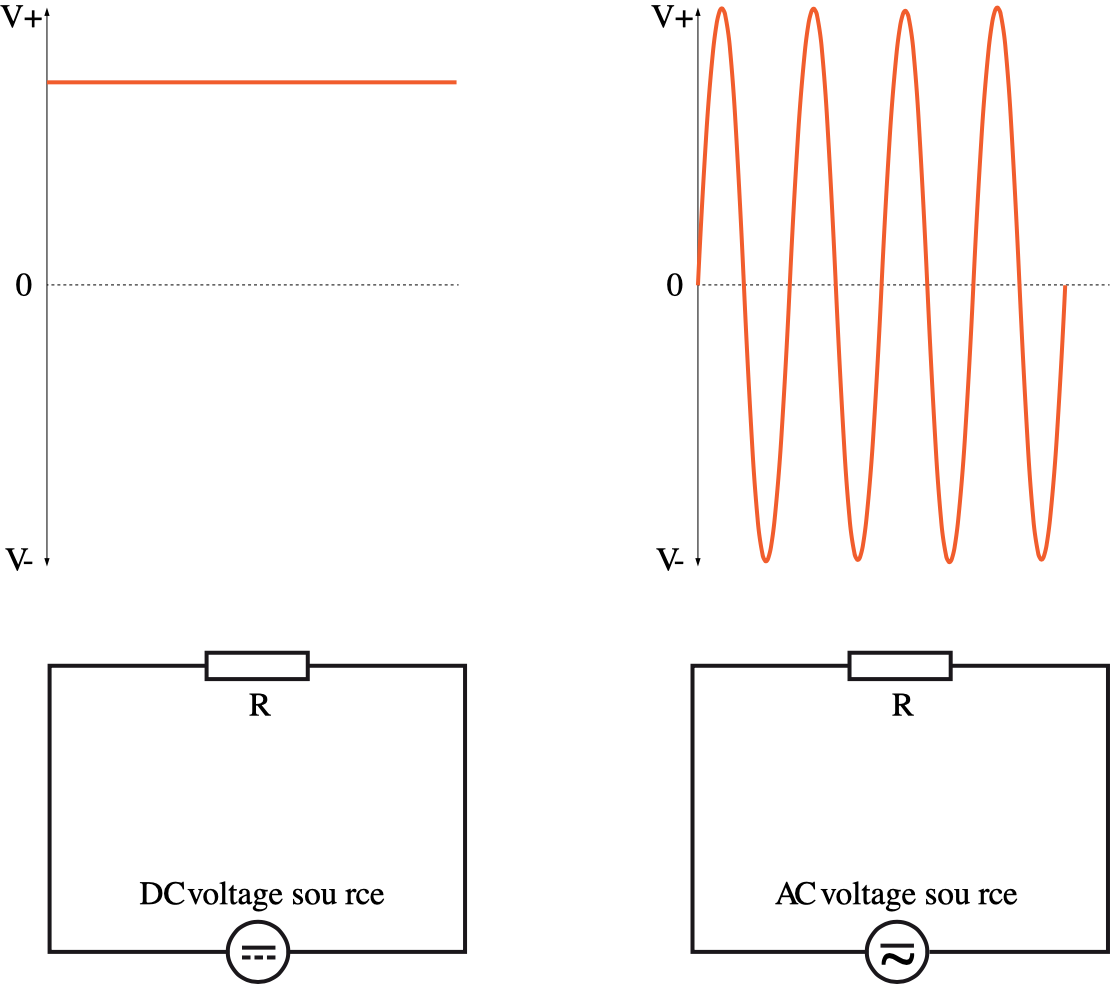

Now it's time to do some practical voltage measurements and have some fun while doing it.

Also, it is important to emphasize how much Dewesoft does autonomously to speed up the measuring experience.

As an example, a simple voltage measurement will be done on a discharging capacitor. Connected to the circuit are two capacitors with rectifying diodes as illustrated in the image below, these are then connected to the grid voltage between the L (live) and N (neutral) conductor cables. This type of connection allows the capacitors to charge with the peak voltage in both polarity directions. This yields around 700 V on both capacitors together. The instrument used in this example is the Sirius LV-HV, the HV channel is chosen for the higher voltages. For discharging the capacitors an input capacitance of 10 farads will be used on the module as the discharging resistor which will be connected to points IN+ and IN-.Image 22: Schematic illustration of a simple voltage measurement on a discharging capacitorThe measurement yields the following result as shown in the image, where the capacitor is instantaneously charged and then discharges exponentially.

Capacitor is instantaneously charged and discharged exponentiallyImage 23: Capacitor charge and discharge measurement

In this example the advantage of the dual core amplifier can be seen. For the voltage that is used the 1200 V measurement range must be taken to perform the measurement correctly, but the voltage on the capacitors fall very fast when they discharge, this will cause a noticeable noise level. 

When the voltage drops under 50 V, meaning into the low voltage spectrum, is when the dual core amplifier starts to shine, as it then switches over and starts measuring in the lower ranges, which greatly reduces the noise. This switch can be seen in the image below, it has been zoomed in to exactly where the switch takes place and the voltage drops under 50 V, and the second core then measures the lower voltage range. 

Dual-core mode enabled measurement is resulting in lower rates of noise in low voltage spectrumImage 24: Dual core measurement of low voltage with a reduced noise level