Angle measurement

An angular position sensor measures the position of a shaft and converts the position to an analog or a digital signal. It calculates the orientation of an object in regards to a specified reference position.

Image 1: Tacho probe as an angular sensor

 

There are many different kinds of angular position sensors that are categorized by supply voltage, output type, sensing range, operating temperature range, packaging type and supply current.

Angular position sensors can be found in a wide area of automotive and industrial applications:

• steering wheel position sensing,
• pedal position sensing,
• throttle position sensing,
• torque sensing.
  
  

When choosing the right angular position sensor we have to be careful to select the right one for our needs:

• output type (analog output, digital output),
• sensing range (±500°/s, ±100°/s, ±60°/s, 360°/s),
• supply current (from 100 µA to 13.5 A).

An angular position sensor measures the angular position of a shaft. Angle sensors can be:

• Inductive sensors 
  Image 2: Inductive sensor

   

• Optical probes
  Image 3: Optical probe

   

• Encoders 
  Image 4: Encoder connected to Dewesoft Sirius device

   

• Gear tooth with missing teeth 
  Image 5: Gear tooth with missing teeth

   

You can connect the following types of sensors to Dewesoft software and hardware:

SENSOR	ANALOG	DIGITAL
Encoder	(relative, absolute is not supported)
Tacho
Geartooth CMD
Geartooth with zero
Geartooth with missing teeth
Geartooth with double teeth	(x-n type sensors)
Linear Encoder
Linear pulses Encoder
Tape sensor

When measuring angle it is critical to select the appropriate sensor to do your measurement correctly.

	ADVANTAGES	DISADVANTAGES	PREVIEW
Encoder	best resolution	critical mounting	Image 6: Encoder
	useful for low RPMs
Tacho sensor	easy installation	bad resolution	Image 7: Tacho sensor
	cheap	not useful for TV and CA
Tape sensor	easy installation	expensive	Image 8: Tape sensor
	good resolution
	zero position
CA-RIE encoder	best for high RPM vibrations	extensive installation	Image 9: CA-RIE encoder

A Rotary Variable Differential Transformer (RVDT) is an angular position sensor that produces an output voltage proportional to the angular displacement.

Image 10: RVDT position sensor

 

When the rotor is in a position that directs the available flux equally in both the in-phase and out-of-phase coils, the output voltages cancel each other out and the result is a zero value signal. This is referred to as the electrical zero position. When the rotor shaft is displaced from the electrical zero position, the resulting output signals have a magnitude and phase relationship proportional to the direction of rotation. Because RVDTs perform essentially like a transformer, the excitation voltages changes will cause proportional changes to the output (transformation ratio). However, the voltage out to excitation voltage ratio will remain constant.

Basic RVDT construction and operation are provided by rotating an iron-core bearing supported within a housed stator. The stator consists of a primary excitation coil and a pair of secondary output coils. A fixed alternating current excitation is applied to the primary stator coil that is electromagnetically coupled to the secondary coils. This coupling is proportional to the angle of the input shaft. The output pair is structured so that one coil is in-phase with the excitation coil, and the second is 180 degrees out-of-phase with the excitation coil.

Image 11: RVDT consists of a rotor and a stator with primary excitation coil and a pair of secondary output coils

 

The output wave form is a sine function. A full 360° rotation of the shaft will result in either one or two sine wave cycles depending upon the RVDT design. These different designs are referred to as either single cycle or dual cycle RVDTs. The usable linear range for the single cycle is ±80° around electrical zero. The linear range for the two cycle is ±40° around the zero, with the two cycle exhibiting higher accuracy. These angular sensors typically provide MTBFs higher than any other type of angular sensor.

The MSI-LVDT adapter is a complete linear variable differential transformer (LVDT) signal conditioning subsystem. It is used in conjunction with the LVDTs to convert transducer's mechanical position to a unipolar DC voltage with a high degree of accuracy and repeatability.

The LVDT converts the position or linear displacement from a mechanical reference (zero or null position) into a proportional electrical signal containing phase (for direction) and amplitude (for distance) information. The LVDT operation does not require an electrical contact between the moving part (probe or core assembly) and the coil assembly but instead relies on the electromagnetic coupling.

The adapter generates 4 or 10 kHz excitation to be able to connect to LVDT sensors and provides phase adjustment with a potentiometer, where the output of 1 V equals 1000 mV/V. It has also an automatic adapter identification.

Functional block diagram of MSI - LVDT

Image 12: Functional block diagram of a MSI - LVDT adapter

 

MSI - LVDT adapter uses a unique ratiometric architecture to eliminate several of the disadvantages associated with traditional approaches to LVDT interfacing. The benefits of this new circuit are: no adjustments are necessary, temperature stability is improved and the transducer interchangeability is improved.

Technical data of MSI - LVDT

MSI - LVDT adapter is powered by EXC voltage. LVDT adapter is compatible with SIRIUS(i) (variable EXC) or DEWE-43A type instrument (fixed ±5V EXC).

Image 13: MSI - LVDT adapter properties 

Operation of MSI - LVDT

Connect the LVDT adapter to your SIRIUS or DEWE-43 channel and connect your sensor probe to SENSOR input.

Image 14: MSI - LVDT adapter

Depending on the sensor used select excitation frequency of the adapter as close as possible to the required one.

With phase compensation, you can adjust the measured output to the maximum output value.

MSI adapters / TEDS sensor support

Since there is an inbuilt TEDS device in the adapter itself and if the MSI adapters/TEDS sensors under Hardware setup is selected, the adapter will be recognized and proper excitation voltage will be set automatically.

Please check if you are using the latest software where the LVDT Adapter is supported.

Image 15: Enable DSI adapters and TEDS sensors in Settings

 
MSI - LVDT adapter is recognized and set automatically.

Manual settings

If MSI adapters/TEDS sensors are left unchecked in Devices settings then the sensor supply and range has to be set manually. Under Channel setup for channel N then set the Excitation voltage from 10V to 15V maximum according to the Image 13.

Image 16: Unchecked option for DSI adapters

 

A tachometer is a sensor device for measuring the rotation speed of an object such as the engine shaft in a car. This device indicates the revolutions per minute (RPM) performed by the object.

• Digital tachometers - comprised of an LCD or LED readout and a memory for storage. These can perform statistical operations and are very suitable for precision measurement and monitoring of any kind of time-based quantities. Digital tachometers are more common these days and they provide numerical readings instead of using dials and needles.
• Contact and non-contact tachometers the contact type is in contact with the rotating shaft. The non-contact type is ideal for applications that are mobile and uses a laser or an optical disk. In the contact type, an optical encoder or magnetic sensor is used.
• Time and frequency measuring tachometers both of these are based on the measurement methods. The time measurement device calculates speed by measuring the time interval between the incoming pulses; whereas, the frequency measurement device calculates speed by measuring the frequency of the incoming pulses. The time measuring tachometers are ideal for low-speed measurements and frequency measuring tachometers are ideal for high-speed measurements.

Working principle and applications

The working principle of an electronic tachometer is quite simple. The system triggers a voltage pulse at the output of the tachometer electromechanical part. The electromechanical part responds to the average voltage of the series of pulses. It shows that the average voltage of the pulse train is proportional to the rotational speed. The signal from the perception head is transmitted by standard twin screened cable to the indicator.

The tachometers are temperature compensated to be able to handle operations in the ambient temperature range of 10°C to +70°C.

Key applications where tachometers are used:

• Automotive - measures the speed at which mechanical devices rotate, which is typically indicated in RPMs. They are used to monitor the RPMs in automobiles because running the engine at excessively high RPM rates can drastically shorten the life of the engine).
• Airplanes - airplanes typically have one tachometer for each engine, and in those that use propellers, one is also needed for each propeller. In the case of aircraft with gas turbines, there are normally at least two tacho sensors there - one for inner high-pressure combustion propeller shaft and another for outer lower-pressure air inflow propeller shaft. A plane's engines usually operate at higher RPMs than its propellers. By using separate instruments for the different parts, the plane's pilot or crew can know whether there is a problem with any particular part).

Dewesoft Tacho Sensors

• DS-TACHO2

Optical tacho probe with LED	Image 17: DS-TACHO2
Stainless steel with 2.5 m cable
up to 4kHz frequency
distance to object up to 1 m
power supply 3 - 15 VDC, 45 mA
Visible red pointer
Control LED
Operating temperature -10°C to +70°C
Dimensions: 73 mm length, 16 mm diameter
L1B7 connector for SIRIUS and DEWE-43 counter input
Including 30 cm reflector band

• DS-TACHO3

Optical Tacho probe with LASER (red class 2)	Image 18: DS-TACHO3
Stainless steel with 2.5 m cable
Up to 4 kHz frequency
Distance to object up to 7.5 m
Power supply 3 - 15 VDC, 0.13 W
Visible red pointer
Control LED
Operating temperature -10°C to +70°C
Dimensions: 73 mm length, 16 mm diameter
L1B7 connector for SIRIUS and DEWE-43 counter input
Including 30 cm reflector band

• DS-TACHO4
  

Optical Tacho probe with LASER (red class 2)	Image 19: DS-TACHO4
With 5 m optical fiber and trigger box
Up to 100 kHz frequency
Distance to object 2 - 5 mm
Power supply 3 - 30 VDC, 120 mA
Operating temperature -10°C to +70°C
Dimensions M6 x 20 mm, 2.5 m cable
L1B7 connector for SIRIUS and DEWE-43 counter input
Including 1 m reflector band with 2 mm black/white grid

Measurement example with tachometer

Measurement example was made with a Tacho probe mounted on a rotating shaft of a machine. On the picture below we can see the signal from the tacho. We get one spike for every rotation of the shaft.

With the Angle sensor math in Dewesoft X, we can calculate the exact frequency and angle from our signal. The input to the math channel was our signal from the tacho (type: Tacho (Digital)). If we take a look at the picture above, we can set the trigger and retrigger level right.

In the measure mode, we add a digital meter to show the frequency of rotations. We can also see the frequency from cursor values (right setup of Cursor I and II).

DS-TACHO1 is a tacho adapter that converts the analog tacho signal to a Dewesoft instrument's CNT / DI input (Lemo 7pin) with an adjustable trigger level (TTL logic signal). Fits to the COUNTER input (Lemo 7pin) on DEWE-43 and SIRIUS ±100V input isolated, trigger threshold adjustable ±10mV ±2V.

Image 23: DS-TACHO1

 

Tacho adapter electronic specifications table:

How does it work?

Connect the DS-TACHO1 with the LEMO 7pin to a DEWE-43 or a SIRIUS Counter input, and on the DSUB 9pin side to your analog tacho probe signal (e.g. magnetic pick up sensor with screw, 1 pulse per revolution).

Start the rotating machine, then use a screwdriver to manually adjust the trigger level on the DS-TACHO1, see picture below.

Image 24: Adjusting the DS-TACHO1

 

When the trigger is detected correctly, the blue LED will flash. Vary the RPM on the machine to check if the trigger level is ok for the whole RPM range.

The lowest detectable frequency for the counter input on the DEWE-43 / SIRIUS is 5 Hz, therefore if you have 1 pulse/revolution, the lowest RPM is 300. If you need to measure lower RPM, you could increase the number of pulses per revolution (e.g. for inductive probe mount a screw every 90° on the rotating disk and then divide a result by 4).

Image 25: Input signal of magnetic tacho probe (coil)

 

In this example, you see the input signal of a magnetic tacho probe (coil), when a screw on the disk is passing by. The higher the RPM, the higher the induced voltage is, so here you have to set the trigger level low (shown in picture ± 10 mV).

The upper red line is the trigger level, the lower orange line is the retrigger level. The signal has to fall below the lower line to be armed for the next trigger again. This even makes it possible to correctly detect a bad signal as shown above!

The sensing distance between the sensor and the gear tooth is influenced by many factors including the gear teeth dimensions, the grade of ferrous metal of the gear and alignment of the sensor to the gear. Typically, larger teeth and slots allow a larger sensing air gap. For best performance, the sensor should be located as close as possible to the target.

Image 26: Working principle of a Gear tooth sensor

 

Hall effect gear tooth sensing makes use of the Hall element to sense the variation in flux found in the air gap between a magnet and passing ferrous gear teeth. A modern approach is to convert the signal from the Hall element to a digital value and then perform signal processing to create a digital output from that effort. If the signal level changes beyond the preset magnitude from the positive or negative peak the output level is changed. This creates a digital zero-speed peak detection speed sensor. It is immune to orientation requirements and can follow the gear speed down to the cessation of motion. It will detect the first edge of the next tooth immediately after power on. The digital signal processing does introduce an uncertainty from quantification that is greater at higher speeds. Extremely demanding timing requirements like those found in crank position sensors may suffer from the loss of accuracy at high speeds.

Image 27: Hall effect gear tooth sensing

 

In order to detect the passing gear teeth with a Hall effect sensor, it is necessary to provide a source of magnetic energy. The simple way to do this is to arrange a permanent magnet in such a way that the axis of magnetization is pointing towards the surface of the gear teeth. As a tooth moves across the surface of the magnet the flux will become attracted to the lower reluctance path provided by the ferrous steel structure. When this occurs the flux density measured by the Hall element between the face of the sensor and the gear tooth increases.

60-2 angle sensor

The 60-2 angle sensor refers to the fact that crank trigger wheel has 58 teeth with 2 missing. This is also known as a 58 wheel.

Image 28: 60-2 Angle sensor

 

The missing teeth are used as identification so that the sensor can recognize the exact angular position of the crankshaft. Having 58 teeth allows a more precise calculation of engine speed compared to a trigger wheel with fewer teeth.

Image 29: Working principle of the 60-2 angle sensor

 

Measurement with 60-2 angle sensor

Below we can see the signal coming from a 60-2 angle sensor. We can clearly see when the sensor is detecting the 2 missing teeth that are used to detect the zero position of a crankshaft.

Image 30: 2 missing teeth are used to detect the zero position of a crankshaft

 

Zoomed in signal of the 60-2 angle sensor looks like this:

Image 31: Zoomed in signal of the 60-2 angle sensor

 

Gyro sensors are angular velocity sensors, that can sense rotational motion and changes in orientation. Angular velocity is the change in a rotational angle per unit of time and is expressed in deg/s (degrees per second).

Image 32: Gyro sensor 

Types of Gyro sensors

• Ring laser gyros (space shuttle, aircraft),
• Fiber-optic gyros (motorboats, race cars, robot balance control),
• Fluid gyros (radio-controlled helicopters. motion sensors),
• Vibration gyros (car navigation, mobile games, digital cameras). Miniature high-accuracy vibration gyro sensor are indispensable.
  
  

Vibration Gyro sensor

• Vibration gyro sensors can sense angular velocity due to the Coriolis force which is applied to a vibrating element. This motion produces a potential difference from which angular velocity is sensed. The angular velocity is converted into an electrical signal output.
  
  
• Manufacturers are using a variety of materials and structures in an effort to devise compact, high-accuracy gyro sensors that have good characteristics:
  • scale factory
  • shock resistance
  • stability
  • noise characteristics
    
    
    Image 33: Vibration gyro sensor structure 
• Working principle
  • Drive arm vibrates in a certain direction.Image 34: Drive arm vibrates in a certain direction
    
    
    
  • Drive arm vibrates in the direction of rotation.

    Image 35: The direction of rotation
    

     

  • When the gyro is rotated, the Coriolis force acts in the drive arm, producing vertical vibrations.
    Image 36: Coriolis force acting in the drive arm, producing vertical vibrations
     
    
    
  • Stationary part bends due to a vertical drive arm, producing a sensing motion in the sensing arm,
    Image 37: Bending of stationary part produces a sensing motion in the sensing arm 
    
    
    
  • Motion of a pair of sensing arms produces a potential difference from which angular velocity is sensed. The angular velocity is converted to an electrical signal.
    
    
    Image 38: Angular velocity is converted to an electrical signal

Gyro sensor applications

The main applications for gyro sensors are:

• Angular velocity sensing - sensing the amount of angular velocity produced, which is the motion itself (sensing of athletic movement).
• Angle sensing - sensing the angular velocity produced by the movement of the sensor itself. Angles are detected by a CPU. The moved angle is fed to and reflected in an application (car navigation systems, video game controllers and mobile phones).
• Control mechanisms - sensing the vibration produced by external factors. This vibration data is then transmitted as electrical signals to a CPU (correcting the balance or orientation of an object).

Optical sensors are electronic detectors that convert light, or a change in light, into an electronic signal. Rugged industrial encoder is an optical sensor that as well works based on a transmission light principle. The very rugged encoder is mounted between the engine and the brake shaft. An infrared beam is emitted and received at the sensor unit, where the customized marker disk is mounted in-between the sensors gate. The slits on the disk interrupt the infrared beam and the receiver then transforms received light to voltage.

The more slits the encoder has, the higher the resolution is:

• 360 slits = 1° resolution (outer diameter 120 mm)
• 720 slits = 0.5° resolution (outer diameter 230 mm)

Image 39: Optical sensor  

Using fiber-optic sensor for angular displacement measurement

The measurement of angular displacements is very important in many fields. For example, in industry it is used to control the direction of cars, the kinematics of robot arms and the tilt angles of aircraft. This kind of measurement can be integrated into precision rotation stages to control the angular positioning of the optical and/or mechanical components.

Optical systems using the triangulation method can be another way to measure angular displacements. This method is based on the light transmitted or reflected by a mirror. In case of miniaturization of these kinds of sensors, they can be fabricated using conventional or silicon-based micro-fabrication techniques. Fiber-optic sensors offer the possibility of reducing strongly the part of the sensor which interacts with the mechanical system.

An encoder is basically a wheel (or a linear bar) with some marks on it. Usually there are encoders having two marks (A and B) with a phase difference of 90 degrees to one another - this is due to determination of the direction of movement. Some encoders has additional zero pulse (ZERO) - one pulse per revolution which can tell us the absolute position of the encoder.

The two signals (A and B) help to determine the direction of the rotation or movement. When input A leads input B, the value is incremented and when the input B leads input A, the value is decremented. The Z or ZERO signal is a single pulse that occurs once during each shaft rotation and can be used to indicate a zero position. 

Image 40: Encoder marks - A and B for direction determination and ZERO as a zero pulse

Image 41: Encoder coupled together with Dewesoft SIRIUS device

There are several encoder modes: 

• The first one is used to measure only the rising edges of input A - this is the so-called X1 mode. 
• The second mode - X2 mode measures the rising and falling edges of an input A. 
• X4 mode measures rising and falling edges of both input signals. 

X2 and X4 modes are extremely helpful if there is a slow movement (for example with linear encoders) because it will actually increase the resolution of measurement by a factor of two or four.

If there is a fast dynamic measurement (like Torsional Vibration) it will sometimes introduce more errors if X2 mode and X4 mode are used. This is because those two modes assume that the gap ratio is exactly 0.5 and that the encoder electronics switches with exactly the same speed between dark and light areas. We can evaluate this error with period and pulse-width measurements.

Image 42: Pulses determination and synchronization

We connect the A signal to SOURCE0, the B signal of the encoder to AUX_CNT0 and the zero pulse to GATE0.

The Filter is also one very important setting to prevent double counts and glitches. We need to set the filter to react a bit faster than what we expect the events, we need to set it a bit slower than expected frequency of the glitches. With a manual switch and a 102.4 MHz base clock, some glitches can be expected.

The optimal settings for input filter are described in the Digital Counters PRO training course - Section: Input Filter.

The red curve on Image 43 shows the digital signal from the switch and the blue curve shows the counter value. The counter value is increased by each transition from low to high.

Image 43:The counter value is without the input filter increased by each transition from low to high

We can see at some points that the values are counted up when there is glitch (no real pulse). This is because a counter can see every glitch (even below 20 nanoseconds) in the signal. Therefore, we need to use a filter to filter out these glitches.

For example, we use the filter of 500 nanoseconds. Filter checks if each pulse is high at least 500 nanosecond. If it is, the counter value is increased.

Image 44: Counting with an input filter of 500 nanoseconds 

Encoders are a component in motion control systems that provide feedback to drives for accurate speed and position control, and specifying an encoder is a task that can appear to be a difficult endeavor. Major encoder manufacturers continue to release new series of encoders and maintain a large fraction of their legacy lines for customers who want to enjoy the freedom of not worrying about their encoder availability. Options within each encoder series also seem to be growing.

When it comes to mounting, the encoder requires the most thought. 

Although, the interface and electrical options within each encoder series seem lengthy, so this decision is up to individual. When you select a drive, the drive specifications will contain the appropriate input options that must be chosen. Encoder mounting is the most significant aspect that divides their identity, and appropriate selection can optimize both the life and performance of the encoder.

Coupling

Image 45: Coupling the encoder

When a flange or foot mount encoder is chosen, it can be mounted to a motor with the use of a coupling and an adapter. A coupling fastens to each shaft through the use of set screws and has spring or mechanical isolation from shock, vibration, or movement in the motor shaft. This is also typically done when an encoder is matched to an older non-standard motor, when a specification of the particular encoder does not exist in ring or hollow shaft encoder, or the shaft movement is too strenuous for a standard encoder to handle.

Isolating the encoder through coupling has several advantages. Using this method of mounting typically provides electrical isolation from the motor. When electrical isolation does not exist, the encoder is susceptible to noise induced by the high currents supplied to and generated by the motor. If there is electrical noise, then the encoder output may have missing pulses, added pulses, or the encoder could get damaged.

Mechanical isolation is also a benefit. Flexible couplings can absorb shaft movement which can allow for installations on older motors or motors that are used in high shock and vibration applications.

Coupling misalignment

Parallel	Image 46: Parallel coupling misalignment
Skewed	Image 47: Skewed coupling misalignment
Angled	Image 48: Angled coupling misalignment

The disadvantages of using couplings are mostly mechanically related. The primary disadvantage of using couplings is the added length required in line with the shaft. Coupling an encoder can add up to eighteen centimeters in line with the motor shaft when you consider the bracket, the shaft gap within the coupling and the encoder housing. Coupling an encoder also adds multiple steps of installation.

When installing a coupling, misalignment in any of the forms has undesirable side effects. Most importantly, the coupling undergoes avoidable stresses. These stresses can eventually cause the coupling material to tear or break.

Lastly, misalignment can have an effect on speed feedback. This effect is similar to that illustrated by the output velocity of a driven shaft. The ripple in velocity can cause drives to fault or goods to be damaged due to excessive vibration.

Image 49: Different shaft angles cause excessive vibration

Direct mount with tether

Direct mounting with a tether places the encoder directly on the shaft of the motor. The encoder does have bearings, so there is no mechanical alignment needed. It also has a rod or sheet steel tether that bolts to the motor face or any fixed object to keep the body of the encoder from rotating.

Motors are driven by different types of voltage sources, and each voltage source induces different types of shaft and bearing currents. To protect the encoder and motor bearings, the shaft of a direct mount encoder is typically isolated by the use of a plastic sleeve between the motor and encoder shaft. Encoders, that do not have the plastic sleeve or insert, rely on the motor for a shaft current solution or another shaft grounding kit accessory.

Matching the appropriate encoder with the motor may be easier with direct mount encoders. With ring kit encoders, the exact details of the motor face are required. Slotted tethers allow for mounting at various radii from the center of the shaft. Shaft installation requires no alignment with respect to a sensor. This means that once the collar is tightened, the shaft portion of the installation is complete. With the use of spring tethers, the impact of sudden shaft movement is absorbed.

Direct mount encoders typically have a larger moving shaft against the encoder housing. This means that there is a larger area at the point of entry to the electronics than you would see in a coupled encoder. Ring encoders have no entry at all through the shaft. Encoder manufactures are constantly developing new ways to improve this situation. One of which is the use of labyrinth seals.

Ring mount encoders

Image 50: Ring mount encoder mounted on machine

Ring mount encoders come in a minimum of two main pieces: the sensor ring and a magnetic wheel. The ring mounts to the drive or accessory end of the motor, and uses pilot dimensions that comply to an NEMA or IEC standard. The wheel is then inserted onto the shaft, and aligned to the sensor embedded within the ring, and fastened into place.

Since the wheel moving inside the ring is picked up by a separately mounted part with no mechanical connection, the sensors can be potted along with the electronics. This is an improvement over direct mount encoders that rely on the integrity of a series of connector and shaft gaskets. Encoders, like these, are seen most often in the paper industry where the air born paper fiber or dust can built up, or in areas in which machine wash down is required.

Liquids also have little effect on the magnetic technology that is typically used in ring encoders. This means that the encoder's moving parts can be partially or entirely submerged.

Ring encoders do not contain bearings. There is an air gap that surrounds the wheel within the ring housing. Momentary shock is much less likely to cause catastrophic damage since shape and pre-load of bearings are essential to providing good quality signals from a coupled or direct mounted encoder. Slight movement in the shaft, as it rotates, does not cause spring force on the bearings and fatigue in tethers or couplings. Ring encoders also take up less space along the shaft the motor. They mount directly to the face of the motor, and the encoder can also have a mounting surface on the opposite side for brakes or gear boxes.

The primary concern in mounting these types of encoders is the alignment of the wheel with respect to the sensor. This is not a factor in coupled or direct mounted encoders since the sensor is aligned by the factory. The quality of the signal is entirely dependent on the installer's ability to properly align the wheel of the encoder. Wheels can also appear to be aligned, but once the shaft moves may go out of alignment. It is essential to make sure that the encoder wheel lies in the center of its radial and axial movement. Different manufacturers provide different instructions for accomplishing this. If this is all done properly, and the application environment matches its ratings, then it will likely operate for many years.

The simple encoder mode can be selected by choosing the Event counting and Basic encoder counting. First let's set up the encoder.
Signal A is CNT_IN0 and Signal B is CNT_IN1. We set the Encoder mode to X1 mode and we set the Input filter to match our highest frequency. Scaling is easy - simply select counts, revs, or degrees from the drop-down menu in the Unit column in Output channels section or enter any other scale factor.

Image 51: Setting up the Encoder mode in Dewesoft X

Now let's take some measurements. The output of the counter is the one that counts up when the signal A leads the signal B, and counts down when the signal B leads the signal A. The positive edges of the signal A are used to calculate the counts.

Image 52: X1 mode encoder counting  

If we choose X2 mode in the setup, the counter will count raising and falling edges of source A, therefore, the resolution will be increased by a factor of 2. Everything else stays the same.

Image 53: X2 mode encoder counting

X4 mode counts the rising and falling edges of signal A as well as signal B. The resolution of the measurements is, therefore, increased by a factor of 4.

Image 54: X4 mode encoder counting 

The zero pulse is used to reset the measurement when a Z pulse is recognized. The only change to the setup is to check the Encoder zero checkbox. This will reset the counter value to 0 when a zero pulse is passed. We also need to set the number of Encoder pulses for internal calculations (360 in this case).

Image 55: Enabling Encoder zero option in Dewesoft X

The picture below shows the operation. The yellow curve is the zero signal, and the white curve is encoder output. When a pulse is detected on the zero pulse input, the counter value resets to 0.

Image 56: When Z pulse is detected the counter value resets to zero 

The picture below is of a zoomed region of the recorder. It shows that the encoder resets the value of the zero pulse and continues to count up the rising edges of the A signal.

Image 57: Zoomed region of the event when encoder resets the value on the zero pulse and continues to count up the rising edges of the A signal 

DS-TACHO4 sensor is a threshold sensor. This is important especially for the proximity detection mode, the most commonly used for rotating: working distance could change with the albedo and/or the form and distance of the target, also, contrast appears as an important parameter: teeth-no teeth, black and white marks. The recommended distance for encoding application is a few millimeters: put the probe close to the target to avoid an incorrect reading resulting from rocking and wagging of the turning part (Descartes optical law); on the other hand, the reflective tape allows for much more than 100 mm. It is highly recommended that you use the adhesives encoders for optimal results.

A few phenomena may affect the detection function, such as a drop of liquid on top of the probe, excessive dust covering the top, more generally, a non-transparent environment for our light source such as: diesel engine sump film ( i.e. carbon is not transparent for the near I.R.). Patented concept implemented in the sensors strongly simplifies mounting and set-ups. Prior to measurement, it is recommended that a detection test is performed, even at low speed, to ensure detection feasibility and determine detection distance required for the sensor.

If impossible to perform a test due to technical reason or mounting specifics, a theoretical method would be to fix the robe at a distance equivalent to the width of the black and width strips to detect- in any event, without exceeding 4 mm.

Fixing and support of the probe will influence an acquisition of the reading. Please be careful regarding vibration. We recommend that you design your supports including appropriate vibration orders studies. The further the probe will be away from the target, the more the TTL amplitude signal will decrease.

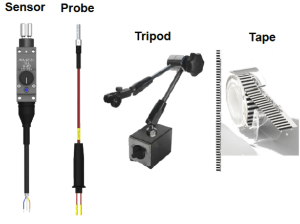
Image 58: DS-TACHO4 bundle

Mounting the Probe

• Ensure that you have all items required at your disposal, i.e. the sensor, the probe, and the two hand-pieces for optical fixation
• Put the two hand-pieces down if they are on the optical head of the sensor
• Insert the two optical fibers with their respective rivets
• Screw the first hand-piece on and tighten moderately; a little gap between the rivet head and the optical head is normal
• Remove the two fibers in order to allow for mounting of the second hand-piece
• Make sure that the two fibers and their rivets are assembled correctly
• Hold both probe and sensor simultaneously when inserting the rubber sleeve to avoid damaging the two optical fibres on the level of the rivets.

Image 59: Proper mounting of the probe 

Adjusting the Probes

The operational mode of the sensor can be seen at the end of the optical fiber by a light beam (not dangerous), which is emitted when the sensor is in 1 mode and not emitted when the sensor is in 0 mode. The sensor keeps its wavelength in near Infra-Red to ensure the power and immunity of the detection function. This also gives an indication of the condition of the optical fiber.

The sensor should be placed about 2 to 5 mm above the tape. A sensitivity potentiometer is available to adjust the trigger level for reliable pulse output.

First turn the potentiometer in mid position. Bring the probe closer to the target until the indicator at the headlights up, targeting the white mark. Shift the probe, and repeat this operation in order to detect the triggering limits on the black marks of the target. Set up the probe in an average position (length), review this operation to confirm the accurate detection: the set up is finished.

Image 60: Adjusting the probe 

Automatic gap detection

When applying the black/white tape to the rotating shaft there will be an irregular rasterization at the transition point. This can be used as the zero pulse to indicate a defined start position. On the other hand, this would result in an rpm drop or spike in our rpm measurement.

A software procedure automatically measures the pulses per revolution and also detects the exact gap length to enable robust and high-quality measurement.

Image 61: Automatic gap detection

The zero pulse must be at least 3 pulses long!

Sensor Setup

Power supply must be perfectly rectified, filtered, and constantly deliver more than 120mA / 12V. This is not an open collector output sensor, but PNP output. 152 G7 can support reverse tension, this tension modifies the signal's amplitude. 152 G7 TTL Voltage output is 5 Vcc, 152 G7 Voltage output is nominal voltage input -1.5Vcc. If the sensor is connected to the acquisition system the use of dedicated measurement connectors and matching cables is recommended. Please refrain from extending the cable. Otherwise, the sensor's operation may be affected. To confirm that the sensor is live, check if a faint red LED glows on the small light channel in front of the sensor optical head; You can also use a digital camera to see the I.R. Light. The brightness of this small red light is independent of the position of the potentiometer.

• Sensor plug-in
   

  V Rating	12 / 24 Vcc	Image 62: Scheme of a sensor
  V Minimal	10 Vcc
  V Maximal	30 Vcc
  Current	120 mA / 12 Vcc

  
  

Image 63: Specifications of a sensor DS-TACHO4

 

• LEMO connector
  • Connector type: L1B7f
    Image 64: 7 pin LEMO connector scheme

     

• Physical diagram

Image 65: Physical diagram of a sensor 

For measuring RPMs and angle at rotating machines, we need angle sensors. RPM and angle measurement is important in balancing, order tracking and rotational and torsional vibration.

We need to choose an RPM sensor that is convenient for our measurement. Not all of the sensors can be installed in our rotating system and sometimes it takes a lot of effort to install them. Also, we have to choose the sensor that has a good resolution for our purpose (e.g.: sensor with one pulse per revolution is not appropriate for measuring precise angle).

The tape sensor is an optical sensor for measuring speed and angle. It uses black and white tape that is attached to the rotating part of a machine.

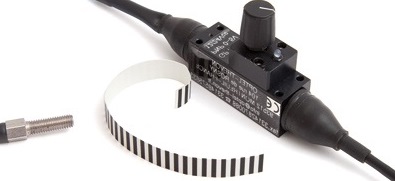
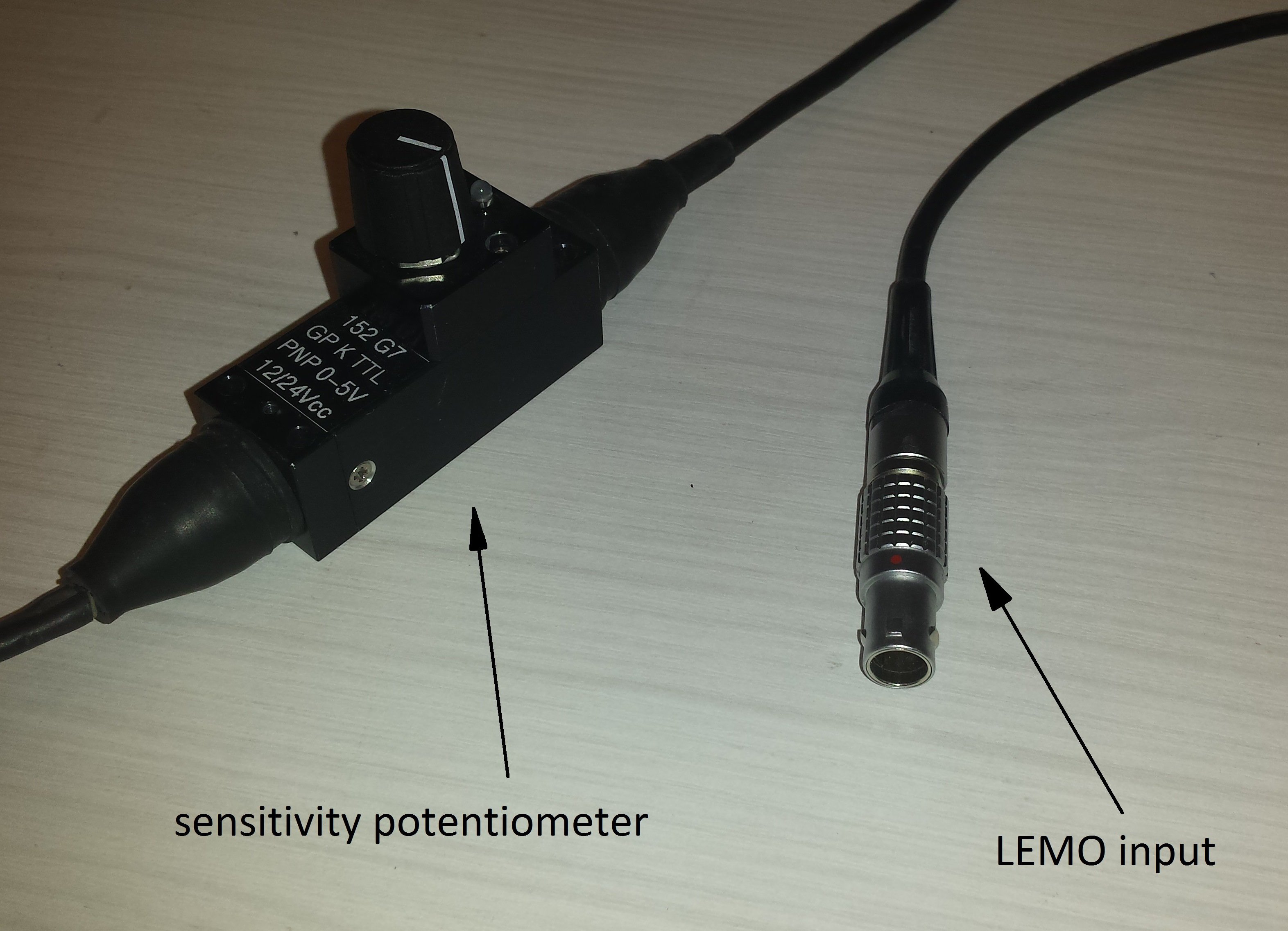
Image 66: Tape sensor with sensitivity potentiometer

 

The sensor is made of optic fibers and should be placed under or about 5 mm above the tape. We have to use a sensitivity potentiometer to adjust the trigger level, which gives us steady pulses. The reflection is then converted from an analyzing electronics into a TTL signal. The sensor is connected directly to a LEMO counter input.

Image 67: Sensitivity potentiometer with LEMO input connector 

A tape sensor can be used in many applications: RPM measurement, angle measurement, order tracking, rotor balancing, rotational and torsional vibration.

Tape sensor Setup

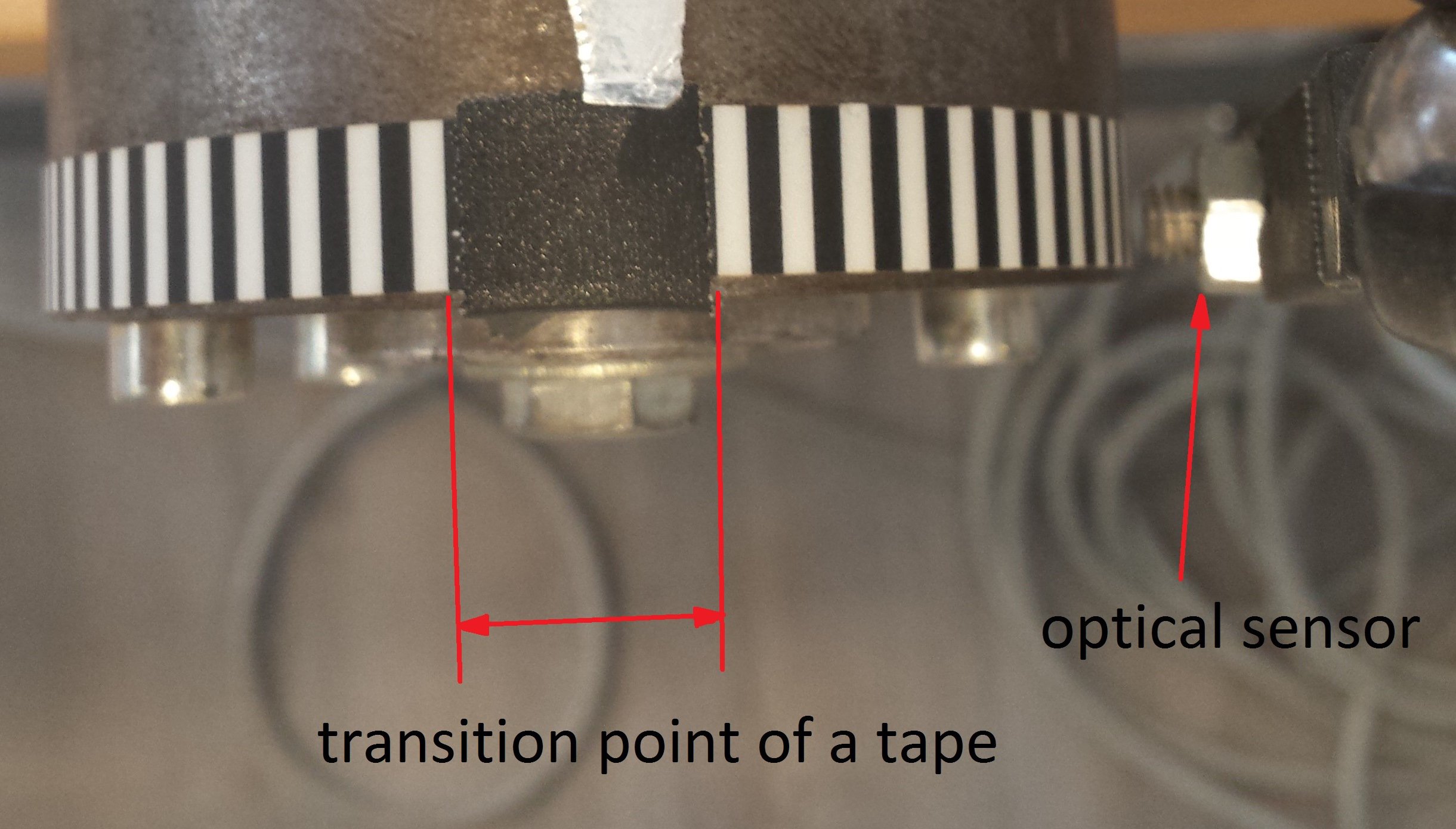
First we glue the tape (with black and white stripes) on our rotating part. If both ends of the tape would come perfectly together we would have no zero pulses per revolution, which is an indication of a start position. If we don't have the information about the start position, the angle would be different at every start of the measurement.

Image 68: Mounting the tape sensor

 

On the picture above we can see the transition point of the tape - we use that as the Zero pulse. This is an indication of a new revolution so the angle will start all the time at this position - angle information related to a shaft will be the same.

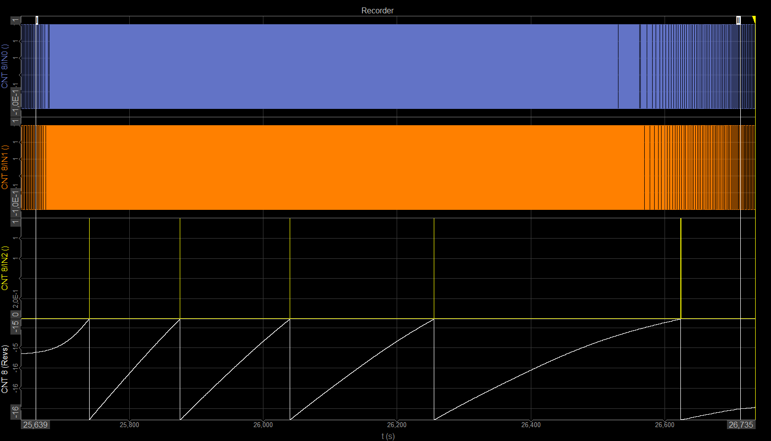
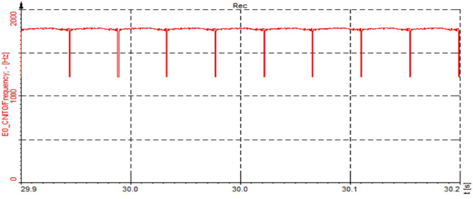
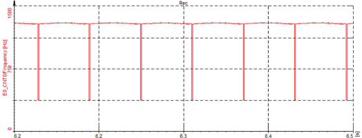
In the picture below we can see the drop in frequency in we have zero pulse. The drop is seen clearly so we could use that to detect the Zero pulse. Angle will always start at that position. For the software to clearly see this drop or peak, the length of the gap must be more than 3 pulses. So the software will have no problem detecting the Zero pulse because the frequency will drop by 70%.

Image 69: Drop-in frequency diagram in case of a zero pulse signal

 

We have to adjust the trigger levels to get reliable pulses from the optical sensor. The trigger level has to be set after the sensor is mounted because it depends on the distance to the tape.

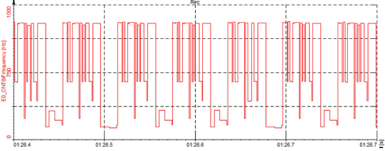
Turn the knob to the left end, and slowly start turning it to the right (clockwise). First there will be no output, as the sensor will not be triggering. After further adjustment, the output will start.

Image 70: Adjusting trigger levels with desire to get reliable pulses

 

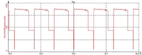
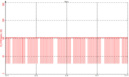
After further adjustment, it will get better and better until we can see the gap nicely.

Image 71: Further adjustment for finding the right gap between pulses

If we make further adjustments it will get worse again as it is shown on Image 72. The right levels are exactly in between.

Image 72: Further adjustments will give incorrect pulses again 

 

The Sample rate must be high enough to detect the frequency drop and that the gap is seen so the software can calculate a start and stop of the angle.

Image 73: Setting up the right Sample rate to detect the frequency drop

 

• Example: We have 64 pulses per revolution and the machine is running at 1000 rpm - 1000 rpm /60 = 16 Hz.
  
  Input frequency is: 16 Hz * 64 pulses/revolution = 1024 Hz. If the sample rate would be set to 1 kHz, the gap would not be recognized at every revolution.
  
  The sampling rate must be at least ten times higher than the maximum input frequency.

Defining sensor Type

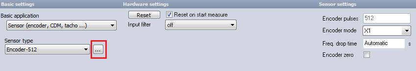
When we do an RPM measurement we have to select Sensor mode in Counter setup in Dewesoft X.

Image 74: For RPM measurements choose Sensor as a Basic application and then select the right Sensor type

 

When Sensor mode is selected, we select our sensor from the Counter sensor database, where types of different sensors and their settings are already stored. If we are using a sensor that is not yet in the Counter sensor database we have to define it.

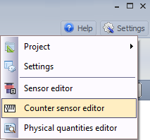
Go to Settings -> Counter sensor editor or just click on the Counter sensor editor:

Image 75: Counter sensor editor

 

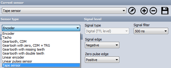
In Counter sensor editor, we add a Tape sensor as Sensor type. Here it is renamed to Tape_sensor. When you click Save&Exit the sensor is added to the Counter sensor database and it is ready to be used.

Image 76: Adding a new sensor in Counter sensor editor

 

We created a tape sensor that can now be selected from the drop-down menu in the counter channel setup:

Image 77: Now select the newly created tape sensor as a Sensor type

 

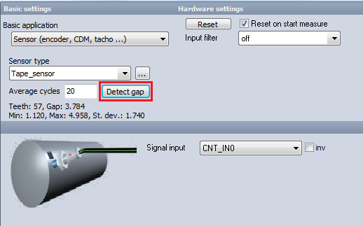
For a precise measurement, we have to know how many pulses per revolution we get from the tape sensor and how many pulses in the gap wide. We shouldn't count them manually, there is a function called Detect gap - it will automatically measure the pulses per revolution and detect the gap length. When measuring gap length the RPMs should be as constant as possible.

The algorithm will average the speed of the machine a few samples before and after the gap, so the average speed around the gap is extracted, and out of that we could calculate the missing pulses.

Measurement results

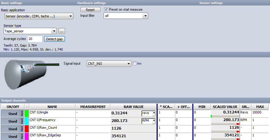
Output channels of the tape sensors are angle and frequency channels. Angle runs from 0° to 360°, frequency channel can be seen in RPMs of in Hz.

Image 78: Output channels of the tape sensors are angle and frequency channels

 

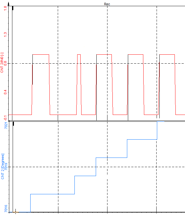
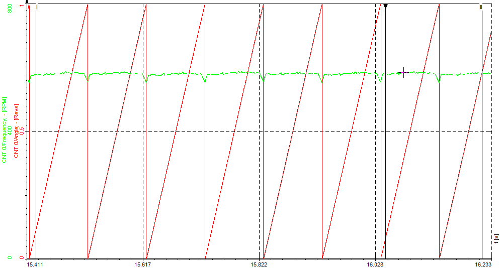
On the recorder we can see the angle in the range from 0° to 360° (when the tape is rotating angle value grows when ZERO pulse is passed, angle value returns to 0) and frequency channel in rpm. The rpm channel (green curve) is not a straight line because our rotor was not balanced. So we can use the tape sensor for balancing rotary parts.

Image 79: When tape is rotating angle value grows, when ZERO pulse is passed, angle value returns to 0 

Counters are mainly used for measuring RPM and the angle of rotating machines. Dewesoft super-counters work on a 102.4 MHz internal time base, ALWAYS, independent of the current sample rate. In comparison to a standard counter, which only outputs whole numbers like 1,1,2,2,3,4 one sample later, Dewesoft X is able to extract the accurate values like 1.37, 1.87, 2.37  fully time and amplitude synchronized! This is done by measuring the exact time of the rising edge of the signal with an additional counter. 

Image 80: Dewesoft Super Counter in comparison with other counters 

Dewesoft supports a lot of different sensor:

Encoder with 1, 2 or 3 tracks (A, B and Z reset signal)	Image 81: Encoder with one and three signal tracks
Linear pulses and pulse encoder	Image 82: Pulse encoder
With an optical tacho probe (1 pulse per revolution) a reflective sticker angle and RPM can be calculated	Image 83: Optical tacho probe
sThe typical automotive sensor, gear tooth with missing teeth (e.g. 60-2) or double teeth, CDM, CDM with zero, CDM with TRG	Image 84: Gear tooth with missing teeth

Frequency/super-counter mode has many advantages over traditional counter measurements.

The problem with traditional counters is that the value of the counter is latched only at the sample rate interval. Therefore, we only have discrete values on each sample. Since the counters can measure exactly where the position of the pulse is between two samples, we can calculate two things out of this: the exact interpolated position of the counter at the sample point, as well as the exact frequency of the pulses.

So how does this mode works? 
The hardware configuration is as follows: we connect a signal (this could be from an encoder, as in an example below) to CNT0.

Now let's set up the channels. For the super-counter and the frequency measurement, we need to use two counters. Another limitation is that the counter channel needs to be an event counter.

The counter is set to Event counting and Basic encoder counting, and then the only thing left is to check the Advanced counter mode. Then the counter pair is set automatically and we have an exact count and an exact frequency as the calculated output channels. The Raw_Count and Raw_EdgeSep are only for advanced purposes - they are raw values coming from the counters.

Image 85: Counting mode setup and enabling the Advanced counter mode option

 

If you look at image 86, we have the Source0, also shown as a digital line (purple) in the upper graph, and in the bottom graph, the orange curve represents the normal counter (raw counter values), which increases the value of each sample. Meanwhile, the white one is the super-counter, where the values are interpolated between the counts, and even more importantly, also between the samples.

• Example: Set the signal frequency from half of the sampling rate up to 50% higher than the sample rate. We will see the normal counter having the same value for the sample, then jumping, then having the same value again, or jumping for two values. The result will be really poor. But if we use the super-counter, the values will be perfectly aligned to the input as shown in the example below. Also, the frequency measurement will be correct.

Image 86: Super-counter values (white) are aligned because of the interpolation between values

 

Super-counter mode is very useful for the run-up and run-down of the test machine, where the super-counter and the frequency are showing perfect measurement results. This is actually the recommended way of measuring all advanced DSA features like order tracking, torsional vibration, and rotational vibration.

We will look at two typical applications in automotive: steering wheel measurements and a wheel speed sensor.

Steering wheel measurement

In this case, a measuring steering wheel with a quadrature encoder sensor is used to measure the angular position and the angular velocity of the steering wheel during test drives. The quadrature encoder used in our example has a resolution of 1800 pulses per revolution.

Image 89: Steering wheel measurement setup 

Channel setup

For the Counter mode, we should select the Sensor(encoder, CDM, tacho...) from the Basic application drop-down menu to decode the signals from the quadrature encoder sensor and select the appropriate sensor (Encoder - ...) from the Sensor type drop-down menu. With Encoder mode, the resolution of the angle measurement can be set. In this example, "X1" is used and the counter outputs 1800 pulses per revolution. X2 would output 3600 pulses per revolution and X4 would output 7200 pulses per revolution. It is recommended to use an Input filter to avoid measurement errors caused by jitters or spikes on the signal (in this case 100ns). The quadrature encoder sensor normally has three signals. Only Signal A and Signal B are used for this application.

It is important that Encoder zero is not chosen if signal Z is connected to the counter input, else a jump in the frequency channel can appear and the manual zero-point definition can be lost. The preferred way is to simply choose the sensor from the list, where all the scaling will be done automatically for us. The Encoder zero has to be de-selected and Reset on start measure should be so as de-selected not to lose the initial zero-point correction.

Image 90: De-select the Resent on start measure and the Encoder zero option 

The first output is the angle, where we can select degrees as units (this could also be revs or counts) and the second output is the frequency, which is already scaled in RPM or Hz.

Zero-point definition

After all the settings in the channel setup are made, the steering wheel has to be set to zero for a specific steering angle. In most cases, the steering angle is set to zero while the car drives straight ahead. Zero definition can be done by pushing Reset in the channel setup. This way, the steering angle is set to zero in that steering wheel position.

Image 91: Click on Reset button to define a Zero position

 

A horizontal test track is recommended for the zero-point definition to avoid a steering angle offset error. It is very important that Reset on start measure is not selected, else the counter value is set to zero at every measurement, and thus the zero-point definition will be lost. The picture below shows the measurement results of the steering wheel.

Image 92: Steering wheel rotation measurement result

A wheel speed sensor or a vehicle speed sensor is a type of tachometer. The wheel sensor is used for high precision measurements of wheel speeds and rotations for test drives. We can also measure traveled distance and speed, but for this we need to know the dynamic wheel radius. The dynamic wheel radius, however, depends on the operating state of the wheel, e.g. road condition, driving conditions, cornering ability, tire pressure, and other factors. Therefore, a precise distance measurement with dynamic wheel radius scaling is not recommended. Instead, we could use either a GPS solution like VGPS or radar/optical sensors.

Image 93: Mounting preview of a wheel speed sensor

We need to set the channel setup for the wheel sensor. This sensor is not defined as a standard in Dewesoft X, therefore, we need to create it with the Counter sensor editor.

Image 94: Adding new counter sensor - sensor selection and definition of number of Pulses per revolution

 After the sensor is created, it just has to be selected in the sensor editor under Sensor type drop down list.

The angle output can be set to revs, degrees, or count. The unit for frequency can be set in Hz or RPM.

Image 95: Selecting sensor type in counter settings

After the counter setup is finished, the math channel setup for travelled distance and velocity can be set.

The first math channel is used to calculate the displacement. This is done with the dynamic wheel radius.

The equation for displacement:

A is angle channel output and it is a signal from the counter. R is a dynamic wheel radius. Displacement has units in meters [m]. On the picture below we can see the equation for the displacement in Dewesoft X. Our angle channel output is named 'CNT8/Angle' and the dynamic wheel radius is in our case 0.25m.

Image96: Adding a formula for displacement

The second math channel is used to measure the velocity of the car. The same dynamic wheel radius is used for this calculation.

The equation for velocity:

F is Frequency channel output and it is a signal from the counter and R is the dynamic wheel radius. Velocity has units in meters per second [m/s]. In the picture below we can see the equations for velocity in Dewesoft X. Our frequency channel output is named 'CNT8/Frequency'.

Image 97: Adding a formula for velocity calculation  

Measured and calculated channels are available in real-time without any hardware or additional wiring. The picture below shows the measurement results from the wheel sensor.

Image 98: Measurement results from the wheel sensor 

Rotating machinery measurements are related to angular and time domain. A correct transformation of collected data in the time domain (accelerometers, pressure sensor,...) to the angular domain (encoder, inductive sensor,...) is important. By using internal clocking on the device, we have the benefit of both:

• time domain data (FFT of vibrations, CAN bus data, voltages, currents,...)
• angular domain data (harmonic components, pressure/position relation,...)
  
  

We are interested in analysing combustion engine in the car to make it more efficient. The task is to measure the position of maximum pressure. This is related to the position of the piston in the cylinder and not a time of measurement. We know the volume of a cylinder and we measure pressure. So it is best to relate work to a position of a piston in a cylinder. And we can do that if we measure one more parameter - angle of the main shaft.

Image 99: Transformation procedure from Time to Angular domain 

Let's show an example. We were measuring power (red signal) and angle (blue signal) in a time domain. There were many cycles recorded. The angle goes from 0 to 359 degrees and then resets back to 0.

Image 100: Measuring angle and power in a time domain 

Now we want to see the power in angle domain. We use the math called Time-to-vector transform.

Image 101: With Time-to-vector transform Math you can transform the time domain into angular 

The input channel is power and the reference channel is the angle (it goes from 0 to 359 degrees). We will calculate Min, Max, and average value.

On the XY recorder, we can see all the cycles together (just select angle as the X and power as Y-axis).

Image 102: Result of all cycles in angle domain 

If we want to show only the average (blue), the minimum (green) or the maximum (red) curve, we choose a 2D graph.

Image 103: Previewing only average, minimum and maximum power values in angle domain