Signal filtering, Signal suppression, Signal processing

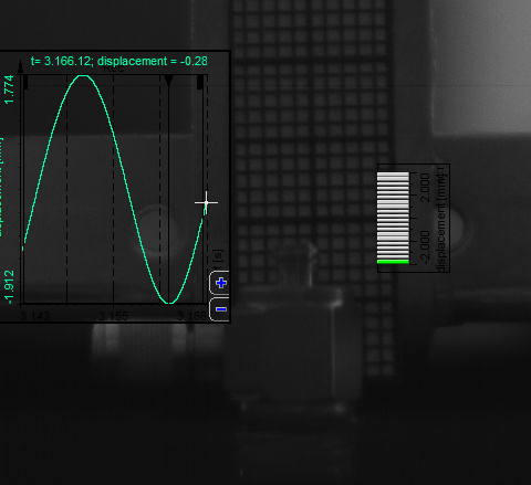
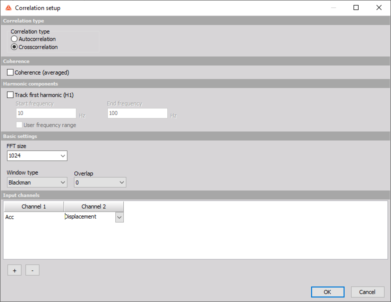
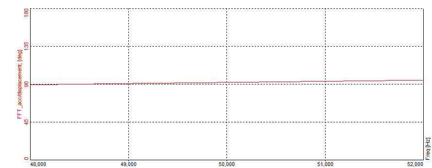
Let's start with some terminology followed by a basic introduction. Then we are going to acquaint ourselves with analog and digital filters, as well as converters and do a comparison of the two. Next on the list will be the different types of filters and their uses. Finally, we are going to see how to setup and use all of these filters in Dewesoft X.

In the field of signal processing, a filter is a device or process that, completely or partially, suppresses unwanted components or features from a signal. This usually means removing some frequencies to suppress interfering signals and to reduce background noise.

Although the task of filters is pretty simple, they are invaluable in today's electronics, particularly in telecommunications.

Terminology

Here is a short list of terms that will be used in this tutorial. Some terms might not be explained here, but will have an explanation later in the text.

• Attenuate - to decrease the amplitude of an electronic signal, with little or no distortion.
• Low-pass filter - a filter that passes low frequencies and attenuates the high ones. 

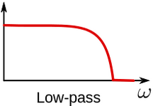
Image 1: Representation of frequency band that is visible after Low-pass filtering

• High-pass filter - a filter that passes high frequencies and attenuates the low ones. 

  Image 2: Representation of frequency band that is visible after High-pass filtering

• Band-pass filter - a filter that passes only frequencies in a specific band. 

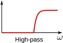
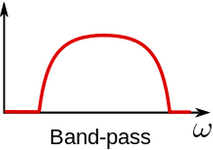
Image 3: Representation of frequency band that is visible after Bandpass filtering

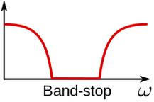
• Band-stop filter - a filter that only attenuates frequencies in a specific band. 

  Image 4: Representation of frequency band that is visible after Bandstop filtering

• Notch filter - a filter that rejects only a specific frequency (an extreme band-stop filter).
• Comb filter - a filter that has multiple regularly spaced narrow pass-bands.
• All-pass filter - a filter that passes all frequencies, but the phase of the output is modified.
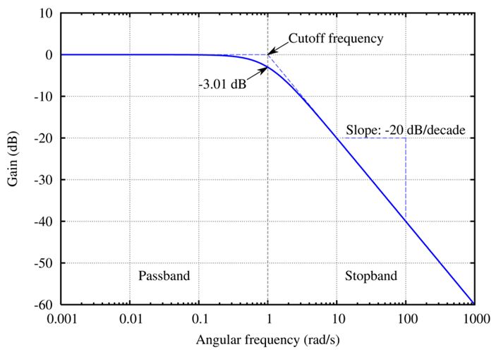
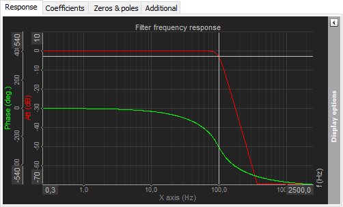
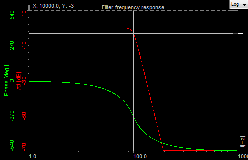
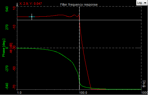
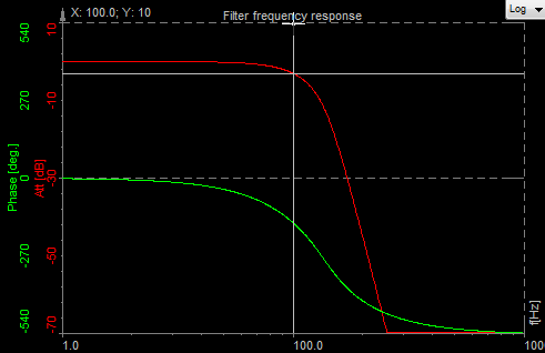
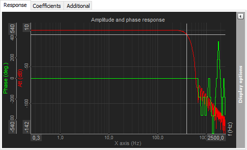
• Cutoff frequency - the frequency beyond which the filter will not pass a signal.
• Roll-off - a rate at which attenuation increases beyond the cutoff frequency. The steepness of the transition between the pass-band and stop-band.
• Transition band - the band of frequencies between a pass-band and stop-band.
• Ripple - the maximum amplitude error of the filter in the passband in dB.
• The order of the filter - the degree of the approximating polynomial (increasing order increases roll-off and brings the filter closer to the ideal response).

Analogue filters are a basic block of signal processing and are designed to operate on a continuously signal (the signal has the value at every instance of time). They are electronic circuits that are dependent on the elements used:

• passive (capacitors, inductors and sometimes resistors),
• active (active elements such as amplifiers combined with passive elements).

They can be linear or non-linear, depending on the type of the equation that describes them. Most analog filters have an infinite impulse response or IIR (this means that the impulse response of the filter, in theory, will never reach zero but in real applications the signal will approach zero and can be neglected). This is because the analog circuit consists of resistors, capacitors, and/or inductors and the latter have a "memory" and their internal state never really relaxes after an impulse.

An example of a 1st order low pass filter

Image 5: Electrical scheme of a 1st order Low-pass filter

 

Digital filter

A digital filter is a signal processing system that performs mathematical operations on a sampled (a continuous signal that has been reduced to a discrete one), discrete-time (unlike the continuous signal, the discrete one does not have a value at every instance of time - it is quantized ), digital (a physical signal that is a representation of a sequence of discrete values - for example, an arbitrary bit stream or a digitized analog signal) signal.

It is used in the same way as analogue filters. They are used to modify a signal (to suppress unwanted parts of the signal).

Filter characteristics:

• type (lowpass, highpass, bandpass, bandstop)
• cutoff frequency
• order (steepness)
• FIR, IIR

  Image 6: Graph of Gain over Angular frequency

  
  

  It can have either a Finite Impulse Response or FIR (the response of the filter after an impulse will reach exactly zero, after a certain, finite amount of time.) or an Infinite Impulse Response (IIR) if feedback is present in the topology of the filter.

A comparison between the continuous and discrete signal:

Image 7:Comparison between the continuous and discrete signal

 

 

 

 

Comparing analogue and digital filters

Analogue filters are much more subjected to non-linearity (resulting in smaller accuracy) because the electronic components that are used for filtering are inherently imperfect and often have values specified to a certain tolerance limit (resistors often have a tolerance of ±5% ). This can be further affected by temperature and time changes. The elements of the circuits also introduce thermal noise, because every element is subject to heating. As we might expect, the more complex the circuit, the greater the magnitude of component errors. On top of that, analogue filters cannot have a FIR response because it would require delay elements.

But where they shine is high-frequency filtering, low latency, and speed. Like it was mentioned in the converter section, a digital filter can not work without preemptive anti-alias filtering, which can only be achieved with a low-pass analog filter. The speed of the analog filter can easily be 10 to 100 times that of a digital one. Also worth mentioning is that in very simple cases, an analog filter surpasses its digital counterpart in terms of cost efficiency.

The digital filter shines in a lot of areas where the analog does not. It is more accurate, supports both IIR and FIR, it can be programmed, making them easier to build and test while giving them greater flexibility. It's also more stable since it isn't affected by temperature and humidity changes. They are also far superior in terms of cost efficiency, especially as the filter gets more complex.

The downsides of digital filters are latency because the signal has to go through two converters and still be processed at high frequencies. In today's modern circuits, both filters are used to complement each other and achieve maximum speed and accuracy.

A comparison of digital and analog filters:

Now that you learned the basics of filters and how they work, we are going to focus only on digital filters and different digital filter types, since the main goal of this tutorial is to teach you how to use them in Dewesoft.

The next chapters will show you how to set appropriate filters in Dewesoft, how to use them and explain what their purpose is. But first, a simple example will show you the usage of filters.

Using filters

Let's find out why we should even use filters. For this example, I have a tuning fork instrumented with strain gage connected on Dewesoft measuring device SIRIUS.

Image 8: DAQ device with strain gage sensor mounted on a tuning fork

 

When the tuning fork is connected to the STG module, it can be seen in Measure mode under Channel setup screen's Analog in section.

Image 9: Analog in channel setup

 

If you take a look at the recorder when a static force is applied on the tuning fork, you can see the changing offset of the signal.

You might also try hitting the tuning fork so it makes a sound that is reflecting the natural frequency of the tuning fork (the conventional way it is used). You can see a high-frequency vibration with falling amplitude because of air friction and friction in the fork.

Image 10: Signal of different forces applied to the tuning fork

 

When looking at the FFT screen (change it to the logarithmic scale to see all the amplitudes), you can see that there is an obvious peak at approximately 440 Hz. You can also place a cursor at this point by simply clicking on the peak in the FFT. The frequency shown is 439.5 Hz. It is not exactly 440 Hz because FFT has a certain line resolution.

This line resolution depends on the sampling rate and the number of lines chosen for the FFT. If you want to have a faster response on the FFT, we would choose fewer lines, but you would have a lower frequency resolution. If on the other hand, you want to see the exact frequency, it is necessary to set a higher line resolution. This is well described in the reference guide, but a simple rule of thumb is: if it takes 1 second to acquire the data from which the FFT is calculated, the resulting FFT will have 1 Hz line resolution. If you acquire data for 2 seconds, line resolution will be 0.5 Hz.

Image 11: FFT and time signal of the vibrating tuning fork

 

This is also a perfect example to learn about using the filters in Dewesoft X. Clearly, there is one part of the signal in the form of the offset (static load) and one part in a form of dynamic ringing with a 440 Hz frequency.

If you want to extract those two components from the original waveform, you need to set two filters - one low pass and one high pass. 

To achieve this add two filters in the Channel setup's Math module.

Image 12: Math made filters

 

1. Setting the 1st filter

• Set by selecting the input channel, in this case, Tuning fork
• Leave Design type at Preset
• In Design parameters confirm that the Prototype is set to Butterworth and set the number of Orders to 6.
• Set the Frequencies filter Type to Low pass, and update Fc2 to 200Hz

This filter will pass all the signals below 200Hz frequency. All the frequencies above 200Hz will be cut off.

2. Setting the 2nd filter 

• Set by selecting the input channel, again to, Tuning fork
• Leave Design type at Preset
• In Design parameters confirm that the Prototype is set to Butterworth and set the number of Orders to 6.
• Set the Frequencies filter Type to High pass, and update Fc1 to 200Hz

This filter will block all the signals below 200Hz frequency and pass by all signals above 200Hz.

If you display those two filters on the recorder, you can see that the signal is nicely decomposed to the static load and dynamic ringing. You can use this technology to cut off unwanted parts of the signal or to extract wanted frequency components of the certain signal.

Image 13: Comparison of RAW, Low-pass filtered and High-pass filtered time signals

 

FIR filter uses only current and past input digital samples to obtain a current output sample value. It does not utilize past output samples.

FIR filter calculates in the way that it takes the input channel data and multiplies it with the specific curve. The easiest example of FIR filter is the averaging filter. Let's say we want to average the input data over three samples. The equation would be like this:

Our simple average filter would have a result like this:

Image 14: Unfiltered and FIR filtered signal

 

The obvious disadvantage is that we would need a lot of input points to be able to filter the data sharp.

IIR filter uses current input sample value, past input, and output samples to obtain current output sample value. We could rewrite the formula like this:

So we are using the previous sample to basically perform exponential averaging, but this very simple and efficient formula will filter the data much more:

Image 15: Unfiltered and IIR filtered signal

 

Comparison of both:

Image 16: Unfiltered, IIR filtered and FIR filtered time signals

 

By the way, these functions were simulated in a Dewesoft X formula by using prev and .data functions:

1. Formula #1. 

Image 17: Math formulas for IIR filter and FIR filter of noise

 

Infinite and finite impulse response

Let's first take a look at the advantages and disadvantages of the IIR response, then the FIR response and finish with a quick summary and overview of both.

The main advantage of IIR filters over FIR filters is their efficient implementation, which helps them to meet specifications in terms of pass-band, stop-band, ripple and/or roll-off. For this, we require a lower order IIR filter, compared to a similar FIR filter. This effectively corresponds to fewer calculations needed, resulting in rather large computational savings. The best use of IIR filters is when the linear characteristics are not of concern and for lower order tapping.

The main disadvantages of IIR are instability, feedback, non-linearity and has limited cycles.

FIR, on the other hand, can make linear characteristics always possible, requires no feedback, is inherently stable, can be easier to design for meeting particular frequency responses and does not have limited cycles. The disadvantage of FIR filters is that they require more memory and computing power than an IIR with similar sharpness or selectivity, particularly when it comes to lower order tapping.

The following table offers a quick comparison of IIR and FIR filter:

Here you will learn how to add a new filter using Dewesoft X.

A new filter can be added inside the Dewesoft X Math module by clicking the Add math button and selecting the appropriate filter from the drop-down menu. You can help yourself by using the search bar, by simply entering FIR, IRR or Frequency domain filter.

We can select the filter type from the following options:

• IIR filter (IIR - Infinite Impulse Response)
• FIR filter (FIR - Finite Impulse Response)
• Frequency domain filter

IIR filters are digital filters with the infinite impulse response, that means that the response to the impulse will be non-zero over an infinite length of time. It supports low pass, high pass, bandpass and bandstop type of filters and multiple input channels. You can select from Chebyshev, Butterworth and Bessel prototypes of a filter. A drawback of the IIR filter is that the phase is not linear.

First, add a new IIR filter in a math section.

In Measure mode go to Channel setup and open the Math module. Search for IIR filter tab and open it.

When you select the IIR filter, the following IIR Filter setup window will open. You can always access this setup window by clicking on the Setup button. On the left side of the setup screen, we have to select the input channel on which the filter will be applied. If we want to apply the same filter to multiple channels we can do that just by selecting all the channels we want to have filtered.

Image 18: Math formulas for IIR filter and FIR filter of noise

In IIR filter setup we can select between two Design types:

• Preset filter (Opened by default)
• Manual filter

The IIR allows High-pass, Low-pass, Bandpass and Bandstop filters.

With filter option on IIR Filter settings section you can set:

• Type and Prototype
• Order
• Cut-off frequency (Low, High)
• Scale
• Ripple (only with Chebyshev filter)

You can see the effects of these settings directly in the Response, Coefficients and Zeros&Poles tabs for Filter Type: Low pass, High pass, Bandpass, Bandstop and different Prototypes.

Image 19: IIR Response curves display

 

Types of filters:

Prototypes of filters:

Order

Cut-off frequency

Fc1 value must be always lower than Fc2. These values are limited by filter stability. In Dewesoft X, the filters are calculated in sections, which enable the ratio between cutoff and sample frequency in a range of 1 to 100000. So we are able to calculate 1 Hz high pass filter with a 100 kHz sampling rate.

Ripple

Scale

This page will offer a brief summary of the three different IIR filter prototypes in Dewesoft X.

Butterworth

The Butterworth filter is a type of signal processing filter designed to have a maximally flat frequency response (having no ripples) on the pass-band and rolls off towards zero in the stop-band. It is also referred to as a maximally flat magnitude filter and offers the smoothest possible curve of any class of filter of the same order.

Image 20: Butterworth filter frequency response

 

Chebyshev

Chebyshev filters have a steeper roll-off and more pass-band ripple (type I) or stop-band ripple (type II) than Butterworth filters. Chebyshev filters have the property that they minimize the error between the idealized and the actual filter characteristic over the range of the filter, but with ripples in the passband. Because of the passband ripple inherent in Chebyshev filters, the ones that have a smoother response in the passband but a more irregular response in the stopband are preferred for some applications.

Image 21: Chebyshev filter frequency response

 

Bessel

Bessel filter is a type of a linear filter with a maximally flat group delay (maximally linear phase response) over its pass-band. The result is a linear phase response, meaning that the passing waveforms will be minimally distorted. It is often used in audio crossover systems. Analog Bessel filters are characterized by almost constant group delay across the entire passband, thus preserving the wave shape of filtered signals in the passband.

Image 22: Bessel filter frequency response 

Let's take a look at the example of a laser output signal, with sharp transitions. We can see the ringing in a signal.

Image 23: Example of a square wave with ringing

The task was, to determine the maximum value of the signal.

First, we use the Butterworth filter prototype (orange). We can see the output of the filter exceeds the maximum value of the signal - the value was wrong.

Image 24: Comparison of raw square wave and Butterworth filtered signal

Then we applied the Bessel filter prototype (green). We can nicely see the maximum value was right at that filter prototype.

Image 25: Comparison of raw square wave and Butterworth and Bassel filtered signals

 

Let's look at the direct comparison between FIR and IIR filter.

Again, let's do the demo with a tuning fork. We connect the forks to STG module. Forks natural frequency is approximately 440 Hz, so set both filters as high-pass filters with cutoff frequency at 200 Hz.

Excite the fork so that it vibrates at its natural frequency.

Image 26: Tuning fork amplitude over time

When you apply FIR filter you can see that there is no phase delay.

Image 27: Aligned phase of Raw signal and FIR filtered signal 

When you apply the IIR filter in the signal, you can clearly see the phase delay.

Image 28: Visible phase delay between Raw signal and IIR filtered signal

On the lower side, you see some useful information about the chosen filter. First is the Response curve.

Image 29: Filter frequency response curve example

The red curve shows the amplification/attenuation of the filter in dB related to the frequency. To refresh the memory, dB scaling is calculated with equation a[dB] = 20 * log10(A), so the attenuation ratio is calculated with A=10^(a/20).

If we read out the value of -34 dB as attenuation, the ratio between input at output at that frequency will be A = 10^(-34/20) = 0,02. So if the input is 1 V sine wave, the output will be 0,02 V sine wave.

The phase (green curve) shows the delay of the signal in degrees.

The lower table shows the coefficients with which the filters will be calculated. The filter is split into several sections for increased stability, so the result from the first section is taken to the next section and so on. These coefficients can be also copy/pasted with the right mouse click on the table to be used from/in other calculation programs.

Image 30: Table of filter coefficients

Zeroes & poles diagram shows the position of filter zeroes and filter poles and can suggest the stability of the filter.

Image 31: Filter Zeroes and Poles

First, add a new FIR filter in a math section.

In Measure mode go to Channel setup and open the Math module. Search for FIR filter tab and open it.

When you press FIR filter the following FIR filter setup window will open. On the left side of the setup screen, you have to select the input channel on which the filter will be applied. If you want to apply the same filter to multiple channels you can do that just by selecting all the channels you want to filter.

Image 32: FIR Filter input field

A nice property of FIR is that the phase response is linear. The phase shift in time is half of the number of samples if the filter is calculated for the samples in the past.

Since Dewesoft X has the calculation delay, we can use the trick to compensate the filter delay and have absolutely no phase shift in pass as well as in the transition band of the filter. This is a major benefit compared to the IIR filter where we always have a phase shift.

For FIR filters you can set:

• Filter type and Window type
• Order (no. of taps)
• Cut-off frequency (Fc1 and Fc2)
• Scale
• Ripple (only with Kaiser window type)

You can see the effect of these settings directly in the Response/Coefficients preview for Filter type: Low pass, High pass, Bandpass, Bandstop and different Window types

Image 33: FIR filter Amplitude and phase response display

Filter type

Window type

The window defines the behaviour of the filter in the transition and the stopband (the height of the sideband and the width of the main band). Window are explained in detail in our FFT guide.

Order

The order of the filter defines the number of coefficients of the filter and that will directly affect the slope of the transition band. The filter order is not directly comparable to FIR filter.

Ripple (only with Kaiser window type)

When a Kaiser Window type is selected, a new Ripple field appears on the right side of the Window type field. In this field, you can enter ripple value in dB. It tells the maximum allowed passband band ripple of the filter. The higher this value is, the bigger will be non-linearity in the passband, but the filter will be stepper.

Cut-off frequency

The filter cutoff frequency defines the -6 dB point (half amplitude) of the filter. You can enter Cut-off frequency in the field:

Fc1 value must be always lower than Fc2. These values are limited by filter stability. In Dewesoft X, the filters are calculated in sections, which enable the ratio between cutoff and sample frequency in a range of 1 to 100000. So we are able to calculate 1 Hz high pass filter with 100 kHz sampling rate.

Scale

For filters, you can enter also Scale. Scale factor means the final multiplication factor before the value is written to the output channel. It helps us to change the unit, for example.

When acquiring analog data with sharp transitions (like square waves) with 24 bit signal-delta ADCs (with an antialiasing filter), we can see some ringing. To eliminate ringing, or at least smooth it out, a FIR filter can be used.

Image 34: Square signal with ringing

If you zoom in the region of the signal at sharp transition.

Image 35: Zummed in region of ringing

First, add the FIR filter. You can find a filter by clicking the Add math button under Math tab as it was described on the previous page.

For best results, this is how you set up the filter:

1. On the left top under Input, select the channel or channels on which the filter will be applied
2. In Design method set the number of Taps to 4
3. Windowing in Design parameters should be set to Blackman 
4. In Frequency settings, use the Low pass Filter type with Fc2 at 1000Hz 

After applying the FIR filter, you can see below that the ringing has been smoothed.

Image 36: Comparison of FIR filtered and unfiltered signal

If you zoom in the region of ringing and compare the signals, original (red) and smoothed (blue) signal, you will notice that the ringing is almost gone and the signal shape has improved.

Image 37: Comparison of reduction in ringing on unfiltered and FIR filtered square wave signal. 

The Custom defined filter setup requires:

• number of sections and coefficients,
• scale factor means the final multiplication factor before the value is written to output channel - for example, it can be used to change the unit,
• individual filter coefficients value.

An FIR filter consists of a single section because it is stable by definition. IIR filters can have several sections.

You define the number of coefficients per section which are a number of rows in the table. This basically defines the filter order.

Image 38: Comparison of 1st order and 10th order filter The last things to define are the filter coefficients. Enter a (input) and b (recur.) values in the z-plane and press the Update button to change the filter settings. You can also copy/paste the coefficients from the clipboard by right-clicking and choosing 'Copy to clipboard' or 'Paste from clipboard' menu item.

Image 39: Table of custom coefficients

The question now is: how to define the coefficient? The answer to this question lies in the knowledge of filter design in s-plane and converting the filter to z-plane.

Usually, the filters are defined in the s-plane. Let's take a simple example of a general formula for a second-order filter:

To get the filter coefficients in the z-plane (time-domain coefficients) you need to use the bilinear transformation:

where fs is the sampling frequency. The upper equation reveals an important fact of filters defined in the z plane - they work only for one sample rate. Therefore, if you need the filters at different sampling rates, the coefficients need to be recalculated.

If you substitute the s in the general formula for a second-order filter with the formula for bilinear transformation, you get:

The first third of the equation is valid for z0 coefficient, second third for z-1 and the third one for z-2. The upper part of the general formula for the second-order filter (with g coefficients) is valid for the input part while the lower part (with h coefficients) is valid for recursive part of the equation.

If you need a higher order filter, you need to make the equation similar to the upper equation with a larger number of the coefficients. The result will have also z-3 factor.

Let's now make a simple example of a second-order Butterworth filter. It has the following prototype in the s-plane:

where the \( \omega_{c} \) is the cutoff frequency in rd/s. You have to adapt the cutoff frequency to the sample rate with pre-warning:

If you write out the factors for this filter from a general equation:

Now let's make the following filter:

• cutoff frequency: fc = 100 Hz
• sampling rate: fs = 1000 Hz

First, you do the pre warping. You can use a technique called pre warping to account for the nonlinearity and produce a more faithful mapping. The warping effect changes the band edges of the digital filter relative to those of the analogue filter in a nonlinear way.

And now you need to calculate the coefficients for the direct and recursive part of the filter with substituting factors in the equation:

Finally, you set the number of coefficients to 3, the number of sections to 1 and enter 6 calculated values in the table and press Update. All entered values are coloured red and button Update also flashes until Update is pressed.

Image 40: Setting a(input)

But you still have to normalize all the numbers to z0 in b(recur.) column (number in row z0 and in column b(recur.) must be set to 1)! To get the right coefficients, all other numbers must be divided with that particular number.

This means that the real values look like this:

Image 41: Setting b(recur)

After entering in all the right coefficients, you have to press the Update button. After updating the red colour will disappear and the filter will be ready to use.

Image 42: Updating the filter

Remember, this is valid only for a sampling rate of 1000 Hz. For others, you need to recalculate the fcp and coefficients.

To make a second-order Butterworth filter it is much easier with Dewesoft X standard filters, but if you need a specific filter, it is necessary to design it 'by hand'.

It is possible to import a custom filter from Matlab (registered trademark of MathWorks company).

To enter the Filter Design & Analysis Tool in Matlab, write fdatool in the Command window.

Image 43: Opening Matlab Filter Design & Analysis Tool

After that, the filter design window will show.

Image 44: Matlab Filter Design & Analysis Tool

Design the IIR filter in Matlab and then click on the filter coefficients button. Filter coefficients should appear in SOS matrix form. That is how they are presented in Dewesoft X.

Image 45: Matlab Filter Design & Analysis Tool

In Dewesoft X, you can't enter the scale factors so you just have to include them in the filter. One section in Dewesoft X equals one SOS section in Matlab. All you have to do is scale it the right way. First three coefficients in Matlab are input and are calculated by multiplying them with the coefficient by the corresponding scale factor. The second three coefficients are recursive and all you need to do is just to copy them from b.

These are calculation formulas for a specific section i:

The coefficients for our example are calculated below:

Image 46: Example coefficients

For the FIR filter, you can choose between Response curve preview and Coefficients display.

The red response curve shows the amplitude damping of the filter. The amplification ratio is expressed in dB (similar to IIR filter). The green curve shows the phase delay. In the passband as well as in the transition band the phase delay is always zero and in the stopband the phase angle is not even important because of high damping ratio.

Image 47: Response curve of the filter

The other display is the display of Coefficients. The upper graph shows the filter coefficients with which the raw data is convoluted. The lower graph shows the response of the filter to the step signal.

Image 48: Coefficients display in filter setup

Let's look at the difference of the FIR filter compared to the standard IIR filter. Let's take a very simple 20 Hz second order filter (at 1 kHz sampling rate).

The IIR filter is calculated with 6 coefficients while similar FIR filter is calculated with 40 coefficients for the same damping. Therefore, the FIR filter is more CPU (central processing unit) demanding for the same performance.

Another fact is while we can get ratios of cutoff frequency to sample rate of 1/100000 and more, we can achieve only limited results with FIR filter. The ratio increases with higher number of coefficients.

Image 49: Comparison of IIR and FIR filters

Let's look at the response graph at 20 Hz (exactly at the limit). The green curve is the original sine wave while the red curve one is calculated with IIR filter. We can clearly see the phase delay of the output.

The blue curve is the response of the FIR filter which has absolutely no phase shift. For lots of applications, it is very important that the signals are not delayed and there the use of FIR filters is very advantageous.

Add a new IIR filter in a math section.

In Measure mode go to Channel setup and open the Math module. Search for Frequency domain filter tab and open it.

When you add the filter or you press the Setup button on the Frequency domain filter line, the following setup window will open. On the left side of the setup screen, we have to select the input channel on which the filter will be applied. If we want to apply the same filter to multiple channels we can do that just by selecting all the channels we want to filter.

Image 50: Example of IIR filter Input selection box

Frequency domain filter description

This filter is quite different than the other types of filters. While IIR and FIR filters are time-domain filters, frequency domain filter calculates the spectrum of the signal with a specific number of lines and overlap and then extracts the RMS value of a certain range of this signal. Therefore, the result is not the full curve, but only one value per frequency spectrum.

The usage of this filter is to extract low peaks of signals where there are big harmonics nearby where it wouldn't be possible to choose IIR filter which would extract low amplitude.

The example below shows the electromotor winding failure which can be seen as low values at the rotation frequency where the line frequency is very high:

Image 51: Example of EM. winding failure

To set the frequency domain filter, it is recommended to observe the signal in the display and choose the right number of lines and a window which fits the best and then set the filter parameters.

Frequency domain filter calculation parameters

Number of lines

This defines the resolution of the filter as well as the number of points in the calculation. The resolution needs to be high enough so that the wanted harmonic can be clearly extracted, but not too high to have a lower result update rate.

Overlap

Overlap defines (same for FFT averaging) how many 'old' data is taken for the next calculation. This increases the result update rate with the same number of lines.

Window type

The window defines the behaviour of the filter in the transition and the stopband (the height of the sidebands and the width of the main band).

Rectangular - the rule of thumb is when we want a pure transformation with no window's side effects (for advanced calculations), we should use a Rectangular window (which is, by the way, equal to no window).

Hamming, Hanning - for general purpose, Hamming or Hanning windows are commonly used because they provide a good compromise between falloff and amplitude error (maximum of 15%). This comes from the fact that old frequency analysers didn't have that many possibilities in terms of frequency lines and these two windows have narrow sideband.

Flat top - if correct amplitudes are searched, we should use the flat-top window. The amplitudes would be wrong by only a fraction (as low as 1%). Of course, there is a penalty - neighbour frequencies are also very high (sideband width is high). Flat top window is most suitable for calibration. But here it is the same: with modern equipment with lots of lines, this is no longer that much of a problem.

RMS amplitude extraction parameters

When filter type is chosen as Tracking, RMS amplitude extraction parameters must be defined.

Frequency source

Fixed - fixed frequency will always take fixed value for the centre frequency.

Tracking - tracking frequency means that the centre frequency will depend on a second input channel (for example rotation frequency).

Centre frequency

If we choose a fixed frequency source, we need to enter the centre frequency in Hz. The centre frequency is the middle value of frequency for value extraction.

Delta frequency

In this field, you can enter delta frequency in Hz. This value depends on the wanted frequency band. It also depends on the window and the number of lines (line resolution).

If we choose Tracking as Frequency source, we need to enter the Frequency channel and Number of harmonics instead of Center frequency:

Frequency channel

Frequency channel is the channel with a current frequency which needs to be extracted. The unit of this channel must be in Hz.

Number of harmonics

When tracking is selected as a frequency source we have to also define the number of harmonics. The number of harmonics describes how many harmonics need to be extracted from the spectrum. If we enter a value of 5, there will be 5 channels created for each input channel. The first channel will have the centre frequency as the frequency channel, second will have twice the frequency of the input and so on.

If Custom filter is selected from the Filter type, then we can design our own filter. With this option, we can create any type of filter curve in the frequency domain and calculate the RMS value. Sometimes it is not easy to define filter characteristics in the time domain, but we have it defined in the frequency domain. Custom FFT filter is perfect for such case.

Image 52: Example of a custom FFT filter

If the frequency source is external, we can define the channel where the frequency is defined and the filter will change the characteristics to always filter correctly like in the time domain. This is especially useful for example for CA noise calculation on the external clock.

Mathematical operations such as derivation and integration are also a kind of a filter. Derivation is a kind of a low-pass filter and integration is a high-pass filter which can also filter DC component.

Derivation

The derivative of a function of a real variable measures the sensitivity to change of a quantity (a function or dependent variable) which is determined by another quantity (the independent variable).

For example, the derivative of the position of a moving object with respect to time is the object's velocity: this measures how quickly the position of the object changes when time is advanced.

The derivative of a function can be geometrically interpreted as the slope of the curve of the mathematical function f(x) plotted as a function of x. But its implications for the modelling of nature go far deeper than this simple geometric application might imply. Its importance lies in the fact that many physical entities such as velocity, acceleration, force and so on are defined as instantaneous rates of change of some other quantity. The derivative can give you a precise instantaneous value for that rate of change and lead to precise modelling of the desired quantity.

The derivate of the function f(x) evaluated at x=a gives the slope of the curve at x=a.

Image 53: Visual representation of derivation

Double derivation

Double derivation of a function f is the derivative of the derivative of f. The second derivative measures how the rate of change of a quantity is itself changing. For example, the second derivative of the position of a vehicle with respect to time is the instantaneous acceleration of the vehicle or the rate at which the velocity of the vehicle is changing with respect to time

Integration

The integral of the function f(x) over the range x=b to x=c gives the area under the curve between those points.

Image 54: Visual representation of integration

The integral gives you a mathematical way of drawing an infinite number of blocks and getting a precise analytical expression for the area. That's very important for geometry - and profoundly important for the physical sciences where the definitions of many physical entities can be cast in a mathematical form the area under a curve. The area of a little block under the curve can be thought of as the width of the strip weighted by (i.e., multiplied by) the height of the strip.

For example, finding the centre of mass of a continuous body involves weighting each element of mass by its distance from an axis of rotation, a process for which the integral is necessary if you are going to get a precise value. A vast number of physical problems involve such infinite sums in their solutions, making the integral an essential tool for the physical scientist.

Double integration

Double integration is useful mainly to directly integrate displacement from acceleration, so use it for dynamic signals

Add a new Integral, derivative math line in the math module.

In Measure mode go to Channel setup and open the Math module. Search for Integral, derivative tab and open it.

Derivation and double derivation is used, as the name already suggests, to calculation derivation of chosen input signals. Here the application range is not divided into two areas since the procedure is similar in all cases. The basic calculation is simple: you subtract the current value from the previous one and divide by the time interval.

Derivation setup

However, this might produce very noisy signals, especially with high sampling frequency. You can look at the derivation of the 20 dB/decade growing filter in the frequency domain. Sometimes it is, therefore, nice to cut the high-frequency contents. You can enable an option to Filter high frequencies and set up the filter by choosing the Order (at least 2 for derivation and at least 3 for double derivation) and High - cutoff frequencies of the signal.

Let's assume the example of calculating acceleration out of the speed of the vehicle. With a car it is a fact that you can't have the acceleration higher than for example 10 Hz coming from the real vehicle acceleration - higher values are basically vibrations. With this in mind, you can choose the 10 Hz as the High frequency and just get the real vehicle acceleration. 

Scale - scaling factor is similar, here the input is divided into second for derivation and divided with second squared for double derivation. So let's calculate the scaling factor for the example above:

km/hour/sec = 1000 m/3600 sec/sec = 0.278 m/s2 = 0.278 / 9,81 g = 0.0283 g

You have to enable Use custom scale and enter this value in the scale field to get correct results.

There are two main purposes of integration: first is to get for example traveled distance from a measured velocity or to get the energy from a measured power. Another type of integration is to calculate the velocity vibration from the measured acceleration.

A clear difference between two basic functions is that in the first application the carrier of information is the DC value - the offset (traveled distance or spent energy). In the other application, the offset is only a measurement error and the carrier of information is the dynamic part of the signal - vibration velocity in our example.

For operations such as integration and derivation, you have to add the Integral, Derivative line from the Add math module. 

Let's first take a look at how to integrate distance from velocity. If you have for example velocity in km/h as an input channel, you select it and switch OFF the option to Filter low frequencies and DC. Now the only thing left is to define the Scale. You have to know that integration adds a sec to the unit

Example: So if you have km/h as input, you have km/h * sec = 1000 m / 3600 sec * sec= 0.278 m. Therefore, if you want to have the output in meters, you have to enter 0.278 as the scale factor. If you want to have the output in km, you have to enter 0.000278. Let's practice on another example - if you have input channel as power in kW, you have at output: kW * sec = kW * 1/3600 * h = 0.000278 kWh - this is our scaling factor.

The second application is to use integration on dynamic signals like vibration acceleration. If you have measured acceleration, there is always some offset because of the amplifier and AD converter offset. This offset will result in a drift of result, which is not wanted, in this case. Therefore, we need to use the option Filter low frequencies and DC to cut this offset.

Image 55: Setting up Integration math

Then you need to define the Order. Be aware that integration is equivalent to a filter with order 1, so you need to choose a high pass filter with order 2 or higher to really cut DC values. The Low tells you where the resulting velocity will be cut off. High values of Low (like 10 Hz) will result in very fast stabilization in the case of overload, but it might on the other side already cut the information we require. Low values (< 1Hz) will result in quite slow stabilization times (typically 5·10 seconds for 1 Hz filter) but will pass through virtually entire frequency range.

For vibration measurement, a usual value is from 3 to 10 Hz for general purpose measurement. For low-frequency vibration like a human body or building vibration, a value between 0.3 and 1 Hz is used. For special application, like seasickness or high structures like TV towers or cranes, that move at a very low frequency, 0.1·0.3 Hz is used. But you have to know that the stabilization will be a very long process. In this case, you also need to make sure that the sensors you are using have such low-frequency range. General-purpose ICP sensors have the cutoff frequency between 0.3 to 1 Hz and, therefore, are not useful in such applications

Let's look at the Scale - scaling factor for this application. Let's assume that you measure the acceleration in g. If you want the results in mm/s, you need to have a scaling factor: 1 g * sec = 9,81 m/sec/sec * sec = 9,81 m/s = 9810 mm/s. So you need to enter 9810 in the field scaling.

Output unit

For output signal from your filter, you can choose from already defined units, if the measured physical quantity is correctly set up.

• m/s
• mm/s
• km/h
• mph
• knot
• ips

Double integration is useful mainly to directly integrate displacement from acceleration, so to use it for dynamic signals. Your output unit will be multiplied by sec*sec. Therefore you need to choose again the option to Filter low frequencies and DC, but you have to take care since the double integration is similar to a second-order filter, you need to choose order 3 or higher for low-frequency filter.

Calculateing the Scale - scaling factor. Usually, you want the measurement result in \( \mu m \) (micrometers). So you have to enter a scaling factor of:

\(  1 g \cdot sec \cdot  sec = 9,81 m/sec/sec \cdot  sec \cdot  sec = 9,81 m = 9,81 \cdot  10^{6}   \mu m \) 

Let's make an example with an accelerometer on a shaker, while recording with a high-speed camera.

Green is the signal from the accelerometer, red is the signal for velocity and blue is the signal for displacement.

You apply the velocity setup (integration setup).

• Operation set to Integration
• Filtered low frequencies and DC enabled, Order set to 2 with Low at 4Hz
• Output unit set to mm/s

Displacement setup (double integration).

• Operation set to Double integration
• Filtered low frequencies and DC enabled, Order set to 4 with Low at 4Hz
• Output unit set to mm

Accelerometer at the top position - calculated displacement is consistent with the actual position of an accelerometer (camera).

Image 57: Calculated displacement and recorded displacement in top position

Accelerometer at middle position - calculated displacement is consistent with the actual position of an accelerometer (camera).

Image 58: Calculated displacement and recorded displacement in the middle position

Accelerometer at bottom position - calculated displacement is consistent with the actual position of an accelerometer (camera).

Image 59: Calculated displacement and recorded displacement in the bottom position

Because integration and derivation is a type of IIR filter, you have a phase delay between signals.

This is an example of how to measure the phase delay between signals. You have to use math called Correlation (add it under math section). You have to calculate cross-correlation between two signals.

Image 60: Using Correlation math to measure the phase delay between signals

Add a 2D graph and apply on the cross-correlation. Select the Complex presentation as Phase (deg). Zoom in to get the phase at the frequency of the shaker (in this case, it was 50 Hz). According to the theory, the phase shift is 90°.

Image 61: Cross-correlation of calculated signals