Sound Level Measurement and Analysis

The sound is a mechanical wave which is an oscillation of pressure transmitted through a medium (like air or water), composed of frequencies within the hearing range. The human ear covers a range of around 20 to 20 000 Hz, depending on age. Frequencies below we call sub-sonic, frequencies above ultra-sonic. Sound needs a medium to distribute and the speed of sound depends on the media:

• in air/gases: 343 m/s (1230 km/h)
• in water: 1482 m/s (5335 km/h)
• in steel: 5960 m/s (21460 km/h)

If an air particle is displaced from its original position, elastic forces of the air tend to restore it to its original position. Because of the inertia of the particle, it overshoots the resting position, bringing into play elastic forces in the opposite direction, and so on.

To understand the proportions, we have to know that we are surrounded by constant atmospheric pressure while our ear only picks up very small pressure changes on top of that. The atmospheric (constant) pressure depending on height above sea level is 1013,25 hPa = 101325 Pa = 1013,25 mbar = 1,01325 bar. So, a sound pressure change of 1 Pa RMS (equals 94 dB) would only change the overall pressure between 101323.6 and 101326.4 Pa.

Sound cannot propagate without a medium - it propagates through compressible media such as air, water and solids as longitudinal waves and also as transverse waves in solids. The sound waves are generated by a sound source (vibrating diaphragm or a stereo speaker). The sound source creates vibrations in the surrounding medium. As the source continues to vibrate the medium, the vibrations propagate away from the source at the speed of sound and are forming the sound wave. At a fixed distance from the sound source, the pressure, velocity, and displacement of the medium vary in time.

Image 1: Propagation of sound through compressible media (air, water, solids, ...)

 

Wavelength and frequency

A sine wave is illustrated in the image below. The wavelength λ is a spatial period of the wave - the distance over which the wave's shape repeats. The wavelength can be measured between successive peaks or between any two corresponding points on the cycle. This is also true for any other periodic wave. The frequency f specifies the number of cycles per second, measured in hertz (Hz).

Image 2: Sine wave with illustrated wavelength and amplitude

 

Sound pressure

Sound pressure or acoustic pressure is the local pressure deviation from the ambient (average, or equilibrium) atmospheric pressure, caused by a sound wave. In the air, sound pressure can be measured using a microphone and in water with a hydrophone. The SI unit for sound pressure p is the pascal (symbol: Pa).

Sound pressure level

Sound pressure level (SPL) or sound level is a logarithmic measure of the effective sound pressure of a sound relative to a reference value. It is measured in decibels (dB) above a standard reference level. The standard reference sound pressure in an air or other gases is 20 µPa, which is usually considered the threshold of human hearing (at 1 kHz). The following equation shows us how to calculate the Sound Pressure level (Lp) in decibels [dB] from sound pressure (p) in Pascal [Pa].

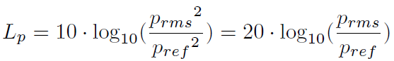
where \(p_{ref}\) is the reference sound pressure and \(p_{rms}\) is the RMS sound pressure being measured.

Most sound level measurements will be made relative to this level. In the air, the reference level is 20 µPa, which equals 0 dB. 1Pa will, for example, equal an SPL of 94 dB. In other media, such as underwater, a reference level (\(p_{ref}\)) of 1 µPa is used, which equals 0 dB.

The minimum level of what the (healthy) human ear can hear is SPL of 0 dB, but the upper limit is not as clearly defined. While 1 bar (194 dB Peak or 191 dB SPL) is the largest pressure variation of an undistorted sound wave can have in Earth's atmosphere, larger sound waves can be present in other atmospheres or other media such as underwater, or through the Earth.

Image 3: Sound pressure level display of the most common noises

 

Ears detect changes in sound pressure. Human hearing does not have a flat frequency response relative to frequency versus amplitude. Humans do not perceive low and high-frequency sounds so well as they perceive sounds near 2000 Hz. Because the frequency response of human hearing changes with amplitude, weighting curves have been established for measuring sound pressure.

In order to take a scientific measurement with a microphone, its precise sensitivity must be known (in volts per pascal - V/Pa). Since this may change over the lifetime of the device, it is necessary to regularly calibrate measurement microphones.

Microphones can be calibrated in two ways. First, we have to know that the direct value of measurement from the microphone is the sound pressure in Pa. Therefore, we need to scale it to the physical quantity.

Scaling with a calibration certificate

If we don't use the calibrator but have the sensitivity of microphones, we can define it directly in the Channel setup.

Image 4: Calibration certificate

 

First, Pa is defined as the physical unit of measurement. Next, we go to Scaling by function, check the Sensitivity and enter the value in mV/Pa, which can be found on the calibration certificate of the microphone.

Image 5: Calibration of a microphone with a certificate in Dewesoft

 

Calibrating the microphone with calibrator

Another way is to calibrate the microphone with the calibrator. In this case, the known parameter is the sound level emitted by the calibrator. The reference calibrator outputs 1 Pa at 1 kHz - from this, we can calculate the dB level.

Image 6: Sound calibrator

 

First, we have to enter the channel setup of the microphone. The sensitivity is set to 1 by default. On the right side of the microphone scaling section, we can see information from the microphone, which is stuck in the calibrator. Calibration frequency is set to 1000 Hz and the current value detected by the microphone is 127.4 dB. This is, of course, wrong because our calibrator has an output value of 94 dB. After we press Calibrate, the sensitivity of the microphone will be measured from the highest peak in the frequency spectrum, usually at 1000 Hz (using of course amplitude correction to get right amplitude).

Image 7: Calibration button to calibrate with sound calibrator

 

After we press the Calibrate button, we can see that the sensitivity has changed. Also, under the current value, we can see the number 94 dB. This means that our microphone is now calibrated.

Image 8: Calculated sensitivity of a microphone from a sound calibrator

 

Microphone sensitivity can also be written on TEDS (Transducer Electronic Data Sheet) chip. In that case, there is no need for calibration.

When we plug the microphone with TEDS into Dewesoft hardware, the sensor is automatically recognized. Measurement mode is set to IEPE and the physical quantity that we measure is sound pressure.

Image 9: TEDS are automatically recognized by Dewesoft

 

In the channel setup, we can see the information about the used microphone. Sensitivity is already written on TEDS, so the microphone is ready to use.

Image 10: Sensitivity of a sensor is written from TEDS

 

There is also other information written on TEDS (serial number, model, manufacturer, calibration data, etc.)

Image 11: Informations read from TEDS (serial number, model, manufacturer, calibration data, ...)

 

In the new version of Dewesoft software, the user can manually calibrate the sensors, even if the sensitivity is written in the TEDS chip.

First press the button with the lock icon to unlock the sensor editor.

Image 12: Lock icon to enter the sensor editor

 

After that, the sensor can be calibrated.

Image 13: Calibration of a microphone with TEDS

 

We put the microphone into the calibrator (94 dB at 1000 Hz) and press the Calibrate button. The new value for sensitivity is calculated.

We can also undo the user calibration with the Undo user calibration button - the sensitivity is restored to the original value, that is written on TEDS.

Image 14: Undo user calibration

 

FFT analysis has a specific number of lines per linear frequency (x-axis) and a CPB (constant percentage bandwidth, called also octave) has a specific number of lines if logarithmic frequency x-axis is used. Therefore, lower frequencies have a higher number of lines and higher frequencies have a lower number of lines. A CPB analysis is traditionally used in the sound and vibration field.

CPB filter is a filter whose bandwidth is a fixed percentage of a center frequency. The width of the individual filters is defined relative to their position in the range of interest. The higher the center frequency of the filter, the wider the bandwidth.

Analysis with CPB filters (and logarithmic scales) is almost always used in connection with acoustic measurements because it gives a close approximation to how the human ear responds.

The widest octave filter used has a bandwidth of 1 octave. Many subdivisions into smaller bandwidths are often used. The filters are often labeled as Constant Percentage Bandwidth filters. A 1/1-octave filter has a bandwidth of close to 70% of its center frequency. The most popular filters are perhaps those with 1/3-octave bandwidths. One advantage is that this bandwidth at frequencies above 500 Hz corresponds well to the frequency selectivity of the human auditory system. Dewesoft supports up to 1/24-octave bandwidth.

A detailed signal with many frequency components shows up with a filter shape as the dotted curve when subjected to an octave analysis. The solid curve shows the increased resolution with more details when a 1/3-octave analysis is used.

Example of a 1/1-octave filter:

Image 15: Example of 1/1 octave filter

 

Example of a 1/3-octave filter:

Image 16: Example of 1/3 octave filter

 

Example of a 1/12-octave filter:

Image 17: Example of 1/12 octave filter

 

A human ear doesn't have an equal "gain" at different frequencies. We will perceive the same level of sound pressure at 1 kHz louder than at 100 Hz. To compensate for this "error", we use frequency weighting curves, which give the same response as the human ear has. The most commonly known example is frequency weighting in sound level measurement where a specific set of weighting curves known as A, B, C, and D weighting as defined in IEC 61672 are used. Unweighed measurements of sound pressure do not correspond to perceived loudness because the human ear is less sensitive at too low and high frequencies. The curves are applied to the measured sound level, by the use of a weighting filter in a sound level meter.

Image 18: Frequency weighting curves

 

• A-weighting: A-weighting is applied to measured sound levels in an effort to account for the relative loudness perceived by the human ear. The human ear is less sensitive to low and high audio frequencies.
• B-weighting: B-weighting is similar to A, except for the fact that low-frequency attenuation is less extreme (-10 dB at 60 Hz). This is the best weighting to use for musical listening purposes.
• C-weighting: C-weighting is similar to A and B as far as the high frequencies are concerned. In the low-frequency range, it hardly provides attenuation. This weighting is used for high-level noise.
• D-weighting: D-weighting was specifically designed for use when measuring high-level aircraft noise in accordance with the IEC 537 measurement standard. The large peak in the D-weighting curve reflects the fact that humans hear random noise differently from pure tones, an effect that is particularly pronounced around 6 kHz.
• Z-weighting (linear): Z-weighting is linear at all frequencies and it has the same effect on all measured values.

The Sound level Math section allows calculation of the typical parameters for sound level measurements from a single microphone. It allows Dewesoft to be used as the typical sound level meter. With appropriate hardware (SIRIUS data acquisition system with ACC amplifier - ICP/IEPE) it can easily fulfill all the requirements for a Class I sound level meter.

It supports different standards like:

• IEC60651, 
• IEC60804, 
• IEC61672.

Sound level meter can be found under Math modules. When you open the SLM, the window appears:

Image 19: Sound level meter channel setup in Dewesoft

 

Basic procedures of Sound level measurement are:

• channel setup
• microphone calibration
• measurement

To use Sound level module, please first select one or more analog channels in the Analog tab to measure the sound.

Image 20: Three microphones connected to analog channels in Dewesoft.

 

Then switch to the Sound level tab. Several modules can be used within a session.

A screen like the one shown below will appear. First of all, select the Input channels that should be measured at the upper left side of the display. In our case, the analog channels are selected. We can select multiple channels and then have several output channels with the same settings.

Image 21: SLM channel setup in Dewesoft with marked different section

1. 1. Input channels
2. 2. Frequency weighting
3. 3. Time weighting
4. 4. Lpk weighting
5. 5. Output time channels
6. 6. Output calculated channels
7. 7. Channel output naming
8. 8. Medium and calibration

Calculation type

We have several options to select from in the Calculation type section. Any combination of Frequency weighting (frequency response to human hearing) and Time weighting (time averaging) can be selected.

Image 22: Frequency weighting options

 

• A-weighting is applied to instrument-measured sound levels in an effort to account for the relative loudness perceived by the human ear, as the ear is less sensitive to low audio frequencies. This is the standard weighting for the sound used in most cases.
• B-weighting is applied to use for musical listening purposes.
• C-weighting is applied for high-level noise.
• D- weighting is applied when measuring a high-level aircraft noise in accordance with the IEC 537 measurement standard.
• Lin(Z)-weighting is linear at all frequencies and it has the same effect on all measured values.

Image 23: Time weighting options

 

Sound level measurements using any grade of a sound level meter can be Fast (F), Slow (S), or Impulse (I) time-weighted. These weightings date back to the time when sound level meters had analog meters and defined the speed at which the meter moved.

• Fast - the needle would move fast to show quickly varying noise. Fast corresponds to a 125 ms time constant.
• Slow - the needle would be damped to smooth the noise out to be easier to read. Slow corresponds to a 1-second time constant.
• Impulse - The Impulse time weighting is about four times faster than Fast, with a short rising time constant but a slow falling constant. Impulse has a rise time constant of 35 ms and fall time constant of 1,5 s.

Image 24: Time weighting comparison

 

We can also select the weighting specifically for Lpk weighting from linear (Z), A, and C. For Lpk calculation we normally use C-weighting even if the overall values are calculated with standard A-weighting.

Image 25: Lpk weighting options

 

Output time channels

We have three types of Output time channels:

Image 26: Output time channels

 

• Lp (SPL) - time and frequency-weighted sound pressure level (SPL) already scaled to dB (decibel) which depends on Calculation type selection -> Frequency weighting and/or Time weighting. For each combination of selection in these sections, one separate output channel is created.
• Lpk value, which shows the current maximum value of the sound levels and depends on Calculation type selection -> Lpk weighting. For the selected choice in this section, one separate output channel is created.
• The frequency weighted raw value shows the frequency weighted time curve of sound in Pa (Pascal). This value depends on Calculation type selection -> Frequency weighting. For each selected choice in this section, one separate output channel is created. This channel can be used for example in frequency analysis or to do further math processing on frequency weighted curves such a detailed classification.

Output calculated channels

Then we need to select Output calculated channels (parameters). These parameters can be Overall values, which means that we have only one value at the end of the measurement and/or interval logged.

Image 27: Overall output channels

 

If we have an Interval logged value, the time interval for logging is defined. For example, if we select to have Interval logging for Leq with 5 seconds intervals, we will get a new value of _Leq after each 5-second period. After that, the value is reset and the calculation is restarted.

Image 28: Interval logging of output channels

 

The values that can be calculated (Output calculated channels) are (these values depend on Calculation type selection -> Frequency weighting and/or Time weighting. For each combination of selection in this sections one separate output channel is created):

Image 29: Calculated channels from SLM

 

• frequency-weighted Leq value, which is equivalent to a sound level
• Lim tells the impulsivity of sound and is the impulse-weighted equivalent; the difference between those two values is calculated as Lim - Leq
• Lpkmax is either C or a linear weighted maximum peak value of sound.
• LE is the frequency-weighted sound energy.
• Lmax and Lmin are the time - and frequency-weighted minimum and maximum levels of sound pressure.
• The next section of sound is classified sound levels. Each calculated value is put in these classes and then we can choose to see LAF1, 5, 10, 50, 90, 95 and 99 % classes of values. To get more details of an e.g. noise situation, the Percentile levels, also called Exceedance levels or Statistical Noise Levels have been introduced. Without looking at the time domain data, one can judge and compare measurements easily when looking at these parameters. For example, a LAF99 value of 40,90 dBA means: during 99% of the time the noise level was 40,9 dB(A). Accordingly, a LAF1 value of 96,20 dBA means: during 1% of the time the noise was 96,2 dB(A). Imagine two measurements: 1) done countryside, where there is only one train per hour passing by. Most of the time the noise level is very low. 2) along the main road, with a lot of traffic noise, with 2000 cars per hour passing by. When LAF90 and LAF10 values don't differ much, this indicates a stable situation. Again, you can choose between two-time bases: LAFx (overall) LAFx_t (interval)

  1 train per hour, otherwise silence	2000 cars per hour
  Image 30: Time-domain signal of silence, 1 train per hour	Image 31: Time domain of a signal with 2000 cars per hour

Medium and calibration

The medium can be selected between air and water. The difference between those two media is in reference to sound pressure. In the air, a reference sound pressure is 20 µPa, and in water, a reference sound pressure is 1µPa.

Image 32: Medium selection in SLM channel setup

 

Calibration of a microphone in Sound level is described on previous pages.

Channel information

Image 33: Channel information in SLM channel setup

 

The lower-left area displays the output channel settings like in the analog setup, like the channel Name, Units, and also Color:

• Name: The first line of a channel name holds the name of the output channel. This name will appear in the channel setup list and in the channel selector for the display. The second line of the channel name usually holds the channel description which will be shown in displays.
• Unit: The units of the channel describe the physically measured units. The default units (mostly dB) are already set.
• Min. and Max. value: The user scale Minimum and Maximum values can be set here. The minimum and maximum scale is used in the display as the default and full display range. The maximum and minimum can be set automatically or manually by entering the value in the fields. Then the max value is not shown in the bar graph since it is displayed in the edit box.

This value is calculated directly in the Medium & calibration field of the sound level module channel setup. We connect the calibrator to the microphone and turn it on. We can see the signal directly in the small overview. In our case, it should be a sine wave with a frequency of 1000 Hz. Since all the frequency weighted curves are referenced to 1000 Hz, this is the usual frequency for calibrating microphones.

We can also choose the medium in which we are measuring. It can be chosen from Air or Water, the difference is in reference to sound pressure.

Image 34: Microphone calibration directly in the SLM setup

 

After we see that the sound is correctly recognized as the sine wave at 1000 Hz, we can click the Calibrate button to perform a calibration. The sound module will calculate the Sensitivity of the microphone from the highest FFT amplitude and reference value.

Image 35: Calibrated microphone directly in the SLM setup

 

The sensitivity will already be directly corrected in the source channel and, therefore, no additional analog scaling is necessary. We can directly check the calibrated sensitivity of the information found on the calibration certificate.

Now we have to check if the calibration was successful. Set a sampling rate of at least 5 kS/s - we would recommend 20 - 50 kS/s - and enter the FFT analysis. Set the FFT options to Flat top filter and the Y scale type to dB Noise. Now press the RMS icon to display the RMS values within the FFT graph. Switch on again your microphone calibrator and the RMS values should display 94 dB.

Image 36: FFT graph of a calibrated microphone

 

If there is a mismatch you should do the calibration again.

The user can specify which time and frequency weightings he wants to combine for sound pressure level, as well as for other parameters. The output format will be the input channel/parameter. To simplify the graphical user interface, the colors at the end of the parameters show which combinations are possible.

For example, in the SoundPressureLevel name Lp the letters Z for linear and S for slow are inserted, resulting in LZSp.

Image 37: Combination of frequency and time weighting for output channels

 

Image 38: Explanation of channel naming

 

As the human ear covers a frequency range from around 20 to 20 000 Hz, we want to measure up to 20 000 Hz. In theory, the sampling rate should be at least two times the highest frequency you want to measure (Nyquist). A typically used sampling rate is 50 000 Hz.

Due to the Sigma-Delta-ADC technology with an anti-aliasing filter, at 50 kHz sampling rate the maximum usable bandwidth is 19531 Hz. The useful range will adapt depending on the selected sampling rate in channel setup, as well as in the FFT instrument.

Image 39: Calculating the bandwidth from the dynamic acquisition rate

 

Image 40: FFT is calculated only up to set bandwidth (according to the Nyquist theorem) 

 

If you need to get a higher resolution for the upper frequency range, you can (currently) go up to 200 kHz with SIRIUS and 1 MHz with SIRIUS-HS hardware.

The True peak level shows the real peak value of the input signal in dB. This should not be mixed up with the maximum sound pressure level! The sound pressure level always contains a time weighting filter, which has an influence on the peak value.

Please see the example below, the raw signal shows a clear maximum at 19,338 Pa, which equals 119,7 dB. The SPL does not reach that high values, no matter if we select F, S or I time weighting. The LCpk however shows the true peak of 120,85 dB. (The remaining deviation is because of the C frequency weighting used here).

Image 41: True peak level without weighting filter in comparison with Sound Pressure Level which has a weighting filter

 

The following table gives an overview of the most commonly used output parameters (not all are shown because of the multiple time/frequency-weighting combinations). The analog input channel was namedMic for this example:

If the interval logging is selected, the Output type of the channels is Asynchronous and the Output rate is custom to the selected interval.

The sound levels module automatically creates a display. We can see the typical screen for sound measurement.

We use the typical A-weighting to calculate Leq (frequency-weighted equivalent continuous sound level) and Lp (time and frequency-weighted sound pressure level), which are shown in the multimeter, bar display, and recorder. Additionally, the octave or narrowband FFT is calculated. This can be achieved by adding an FFT screen and on this screen where we can define frequency weightings, such as A-weighting and dB scaling.

Accordingly, when using more sound level modules (added with the plus button), there will be a screen for every instance (called Sound level meter, Sound level meter 2, etc).

Image 42: Auto-generated measurement screen from Sound Level module

 

During the measurement, we can also change CPB options.

Image 43: CPB widget with options

 

The analysis type defines the width of each band. The next band is calculated as 2^(AnalysisType) from the previous band. For 1/1, this is 2^(1/1)=2, for 1/3 analysis this is 2^(1/3)=1,26 and so on.

For 1/3 spectrum, there will be 10 bands per decade, for 1/12 there will be 40 and for 1/24, there are 80 values.

Y scale type can be chosen between:

• Lin
• Log
• 0 dB
• Sound dB
• Ref. dB

Dewesoft supports two display band types that can be selected from drop-down menu (bars or lines) and is selected according to your application.

Weighting is described in the Frequency weighting page.

When Averaging is enabled, you can choose between Lin, Exp or Peak. The averaging mode is used to get a more stable Octave display.

To activate the averaging just click the Enable checkbox on the Averaging section and all controls become available.

Averaging means that we calculate many FFTs during the time and are averaging the frequency lines.

• linear averaging (each FFT counts the same in the results),
• exponential (FFTs becomes less and less important with time),
• peak hold (only maximum results are stored and shown).

Depending on the application, it may be necessary to define a data overlap. When the window type is used, we have to use an overlap otherwise some of the data will be ignored. Therefore, the use of overlap is highly recommended. Overlap defines how much of the old data will be taken into account.

It takes some part of the time signal, which is already calculated and uses it again for calculation. There could be any number for overlap, but usually, there is 25%, 50%, 66.7%, and 75% overlapping.

50% overlapping means that the calculation will take half of the old data.

There are two ways for octave calculation/visualization of the Sound Pressure Level: 

• Octave preview widget
• Octave analysis math

Octave preview widget

The quickest way is to do the visualization with the widget called Octave preview. You only need to set the y-axis to Sound dB to display the result.

Further options are 1/1, 1/3 up to 1/24 octave resolution; weighting (A, B, C, D, Lin); Averaging (Lin, Exp, Peak) with overlap (0 to 75%).

Image 44: Octave preview widget

 

Octave analysis math

In order to make a math channel with Octave analysis math, you need to add new math.

Image 45: Octave analysis math setup

The result of Octave analysis math is displayed on a 2D graph.

 

Image 46: Results from Octave analysis math are displayed on 2D graph

 

 

 

A very common diagram is also the Sound Level waterfall diagram, where the FFT is displayed as Octave. First, add an Octave analysis function in the math. Then make a math formula for calculating the SoundLevel for each octave band by the formula 20*log10(('mic/CPB')/0.00002). The array mathematic will automatically take care of the data format.

Image 47: Formula for transforming CPB from Pa to dB

 

In the Measure mode, you can then display the array function in the 3D graph. The Octave plots will run through in real-time continuously. With the history count, you can increase the shown buffer.

Image 48: Displaying the CPB time history on a 3D graph

 

As with any other module in Dewesoft, Sound Level can also be calculated offline. You only need to store the raw signals and you can do all calculations afterward on the stored data file.

The procedure can be similar to this: Open the data file, go to Math, go to the Sound Level module, change parameters, click on Review and then on the button Recalculate.

Waterfall FFT - extracting single lines

After you have recorded the waterfall FFT (this feature also works live during measurement), you may want to look at specific octave bands and visualize their time-dependent course as single lines in a recorder.

To extract the single lines of the 3D waterfall, please go to Design mode, right-click on the 3D graph, select Info channels from the context menu and enable both X cut and Y cut.

Image 49: Enable X and Y cut on 3D graph

 

New channels will be generated and shown on the channel list.

Please get a new 2D graph widget from the instrument toolbar in design mode and assign one of the channels to it. Then exit design mode and left-click on the 3D graph on a frequency you are interested in. The info channel in the 2D graph will automatically update because it is linked to the 3D graph.

To remove a marker in the 3D graph, right-click on it.

Currently, only one marker is supported. Multiple markers will show up, but the cut is only done on the position of the first marker.

Image 50: X and Y cut from 3D graph displayed on the 2D graph

 

Acoustic replay/analog out

Any recorded channel can be replayed through the loudspeakers or via Analog out voltage 0...10V (e.g. SIRIUS MULTI module or AO8 option).

Please open a data file, click on the loudspeaker symbol, select the channel you want to hear and click on Play. The replay speed can also be changed.

Image 51: Sound channel replay

 

Printing a report

When the calculations are finished, there are multiple options on how to export the data out of Dewesoft. We can either print the current display arrangement, export to the clipboard or to external software. For the first option just click on the button Print, and select the printer, which can also be a PDF.

For the first option just click on the button Print, and select the printer, which can also be a PDF.

Image 52: Print the report from the measurement screen

 

Export instrument data to the clipboard

A quick way to export the data is by using the clipboard. Click on the widget, e.g. the Octave plot showing the Sound Level data, to set it active. Then select Copy to clipboard -> Widget data from the Edit menu.

Start Excel (or any other program) and paste the data into, the columns and rows will be filled exactly with the data you see.

Image 53: Copy data from selected widget to the clipboard

 

Export to Wave, Matlab, Excel, ...

You can also use the default export into a lot of different file formats, such as Matlab, Excel, Diadem, RPC III, CSV, etc.. For Flex pro and Excel, there is also ActiveX support, providing export into predefined templates for one-click-report generation.

For FlexPro and Excel, there is also ActiveX support, providing export into predefined templates for the one-click-report generation.

Image 54: Export section and supported formats