Strain Measurement Using Strain Gage Sensors

Strain and stress are the results when it comes to external forces that are applied to a non-moving object.

Strain

A strain is defined as the amount of deformation that an object experiences compared to its original size and shape (the ratio of increase in length regarding original length)

The term strain is in most cases used to describe the elongation of a section.

Strain can be caused by the effect of a force.

A strain is a dimensionless quantity and is usually expressed in percentage. Typical measures for strain are less than 2 mm/m for steel and are often expressed in micro-strain units. One microstrain is the strain producing deformation of one part per million.

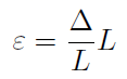
Image 1: Strain is defined as the amount of deformation that an object experiences compared to its original size

 

Stress

Stress is defined as applied force per unit area

It usually occurs as a result of an applied force but is often due to the effects of force within a material or within a larger system.

For example, let's imagine a wire that is anchored at the top and hanging down. We apply weights to the end of this wire to pull it down, thus applying a downward force. We can see that in the picture below, where A is the original cross-sectional area of the wire, and L is the original wire length. In this example, the material (wire) experiences stress which is called the axial stress.

Image 2: Wire that is anchored at the top and hanging down

 

The units are the same as the pressure because the pressure is the special variation of stress. Despite that, stress is still a more complex quantity than pressure, because it fluctuates with direction and with the surface it acts on.

We can calculate the stress (σ) by multiplying strain (ε) and Young's modulus (E).

Force

Therefore

The use of these equations is demonstrated in section section 22.

The connection between stress and strain - Young's modulus.

The Young's modulus, also known as the tensile modulus or elastic modulus is a measure of the stiffness of an elastic material and is a quantity used to characterize materials.

It is defined as the ratio of the stress (force per unit area) along an axis over the strain (ratio of deformation over initial length) along that axis in the range of stress in which Hooke's law holds.

A material, whose Young's modulus is very high, is rigid.

The Young's modulus [E], can be calculated by dividing the tensile stress by the extensional strain in the elastic (initial, linear) portion of the stress-strain curve:

where

• E is Young's modulus (modulus of elasticity)
• F is the force exerted on an object under tension;
• A0 is the original cross-sectional area through which the force is applied;
• ΔL is the amount by which the length of the object changes;
• L0 is the original length of the object.

By the International System of Units, (SI), the unit of Young's modulus is the Pascal (Pa or N/m2 or kg/ms2). The practical units used are megapascals (MPa or N/mm2) or gigapascals (GPa or kN/mm2).

In the United States customary units, Young's modulus is expressed as pounds per square inch (psi).

Measuring modulus of elasticity

Modulus of elasticity and yield stress are two frequent material properties that can be calculated from performing tensile tests with a mechanical testing system.

The procedure of Mechanical testing systems is that the selected material is clamped between two grips. The bottom grip is tightened on the surface while the top grip moves up at a certain displacement rate.

The testing system records the force that is needed to stretch the material and the suitable displacement of the grips. Engineers measure the original cross-sectional area of a specimen and the original length between the grips. After that, they are able to calculate stress from the force data and strain from the displacement data. All the data is then used to create stress-strain diagrams as shown in the image below.

Image 3: Stress-Strain curve

 

1. Normal stress

We know two normal stresses - Tensile and Compressive stress. Tensile stresses are positive, compressive stresses are negative.

Normal stresses arise when tensile or compressive forces act against one another.

1.1 Tension

On the picture below we can see a tensile load applied to a rectangular solid. The response of a rectangular solid to tensile loads is very dependent on the tensile stiffness and strength properties of the reinforcement fibers since these are far higher than the resin system on its own.

Image 4: Tension

 

1.2 Compression

The figure below shows a composite under a compressive load. Here, the adhesive and stiffness properties of the resin system are crucial, as it is the role of the resin to maintain the fibers as straight columns and to prevent them from buckling.

Image 5: Compression

 

2. Shear stress

The figure below shows a composite experiencing a shear load. This load is trying to slide adjacent layers of fibers over each other. Under shear loads, the resin plays a major role, transferring the stresses across the composite. For the composite to perform well under shear loads the resin element must not only exhibit good mechanical properties but must also have high adhesion to the reinforcement fiber. The interlaminar shear strength (ILSS) of a composite is often used to indicate this property in a multi-layer composite ('laminate').

Image 6: Shear stress

 

Image 7: Tensile, compressive, and shear strain

 

Strain gage

A Strain gage is a sensor whose resistance varies with applied force and is commonly used for load, weight, and force detection. It is basically a foil resistor, whose line resistance is proportional to the length and inversely to the area of the cross-section. It consists of a small diameter wire, that is attached to a backing material (usually made of plastic). The wire is looped back and forth several times to create an effectively longer wire. The longer the wire, the larger the resistance, and the larger the change in resistance. However, the change of the resistance is very small, so we need a good amplifier and measurement principle to detect such small differences. It is one of the most important tools of the electrical measurement technique applied to the measurement of mechanical quantities. Strain gages, that are glued to a larger structure under stress, are named Bonded gages. Typical strain gages have a resistances range from 120 Ω to 350 Ω (unstressed) and are smaller than a postage stamp. This resistance may change only a fraction of a percent for the full force range of the gage, given the limitations imposed by the elastic limits of the gage material and of the test specimen. Forces great enough to induce greater resistance changes would permanently deform the test specimen and/or the gage conductors themselves, thus ruining the gage as a measurement device. That's why, in order to use the strain gage as a practical instrument, we must measure extremely small changes in resistance with high accuracy. The ideal strain gage would undergo the change in resistance only because of the deformations of the surface to which the sensor is coupled. However, in real applications, there are many factors that influence detected resistance such as temperature, material properties, the adhesive that bonds the gage to the surface, and the stability of the metal.

Image 8: Strain gage

 

Gage factor (GF or k)

If a wire is held under tension, it gets slightly longer and its cross-sectional area is reduced. This changes its resistance (R) in proportion to the strain sensitivity (S) of the wire's resistance. When a strain is introduced, the strain sensitivity, which is also called the gage factor(GF), is given by:

General examples of strain gages:

The gage factor does not rely on the temperature, however, it is important to know, that it only relates the resistance to the strain if there are no temperature effects. The ideal strain gage would only change resistance due to the deformations of the surface on to which it was attached.

Image 9: Strain gage measurement

 

1. Selection based on gage length:

First, let's explain what is a gage length.

Gage length is the distance along with the specimen upon which extension calculations are made. The gage length is sometimes taken as the distance between the grips.

It ranges from 0.2 mm to 100 mm, but a length of 3 mm to 6 mm is generally recommended for the common applications.

Select a shorter gage (< 3mm) if you are limited to mounting space if a localized strain gradient needs to be measured (on a fillet, hole, or notch with a small diameter (< 25 mm), or if accuracy isn't critical.

Select a longer gage (> 6mm) if you need to install gage really fast. If the gage is longer it is easier to install it, if heat dissipation is an issue (longer gage is less sensitive to heat), if the measured object has non-homogeneous material properties, such as concrete, if you want to save money. Gages with a length of 5.0 - 12.5 mm are usually less expensive than gages of other lengths.

2. Selection based on gage resistance:

The electrical resistance of a strain gage is directly related to its sensitivity. The higher is the resistance, the higher is then the sensitivity.

Select a higher resistance gage (350Ω or 1000Ω) if you need to have higher sensitivity if you need certain compatibility with existing instrumentation.

Select a lower resistance gage (120Ω) if fatigue loading is an issue. Here it is really important to know, that lower resistance wire is larger in diameter, and more fatigue resistant. You can also choose this type if the cost is an issue because 120Ω gages are usually less expensive than 350Ω gages.

3. Selection based on gage pattern:

Before we start explaining gage patterns, it is important to explain what are Strain rosettes.

Strain rosette

A single strain gage can only measure in one direction. To overcome this, we use a strain gage rosette. It is an arrangement of two or more closely positioned gage grids, separately oriented to measure the normal strains along different directions in the underlying surface of the test part. Rosettes are designed to perform a very practical and important function in experimental stress analysis. It can be shown that for the not-uncommon case of the general biaxial stress state, with the principal directions unknown, three independent strain measurements (in different directions) are required to determine the principal strains and stresses. And even when the principal directions are known in advance, two independent strain measurements are needed to obtain the principal strains and stresses.

Image 10: Strain rosette

 

Gage pattern refers to the number of grid and the layout of the grid.

Select a uniaxial strain gage if you need to measure only one direction of strain or if you are limited with money because two or three single uniaxial strain gages are usually less expensive than a bi-axial or tri-element strain gage.

Image 11: Uniaxial strain gage

 

Select a bi-axial strain rosette (0°-90° Tee rosette) if you need to measure principal stress, which means that principal axes are known.

Image 12: Biaxial strain rosette

 

Select a three-element strain rosette (0°-45°-90° rectangular rosette or 0°-60°-120° delta rosette) if you want to measure principal stresses and you don't know the principal axes.

Image 13: Rectangular strain rosette

 

Image 14: Delta strain rosette

 

We know two different layouts in multi-axial strain rosettes: planar and stacked.

Select a strain rosette with planar layout if you have problems with heat dissipation or you have critical accuracy and stability. The planar layout has each gage closer to the measuring surface and no interference in between.

Select a strain rosette with a stacked layout, if the strain gradient is large. Stacked layout measures strain at the same point or if you are limited in mounting space.

Image 15: Delta strain rosette

 

Image 16: Delta strain rosette

 

The mounting of the strain gage is not a difficult task if we follow the suggested procedure. Strain gages are fragile and can be damaged easily.

For mounting a strain gage we need an illuminated magnifier, electrical grade solder, rosin soldering flux, epoxy adhesive, cyanoacrylate adhesive, lacquer thinner, acetone or alcohol, masking tape, toothpicks, tweezers, awl, ruler, fine gage tinned-copper lead wires and ohmmeter.

Important: never touch a gage with your fingers!

Let's take a look at the Youtube video below, which will show us how to install a strain gage.

The video was created by Mechatronics department at the University of Jordan.

Strain gage installation

A short story about the strain gage connections really fits in this context.

Most people are likely familiar with Murphy's Law. It originally states that "Whatever can go wrong, will go wrong". This is very well known, but what is not known so well is that it originates from the strain gage measurements. The "inventor" of this law, Capt. Ed Murphy made a strain gage measurement system for a g-force testing system at Edwards Air Force Base, where the maximum g force, that the human body could take, was to be tested. As a side-note, a real human was used, and the maximum force was 40 g.

The result of the first measurement was zero, simply because the strain gages were connected in such a way that they canceled out each other. Capt. Ed Murphy blamed his assistant for the error, who had connected the gages in the wrong way. The other, even more interesting part of the story for the process of measurement was that Murphy simply declined a verification of the system, which was offered to him before performing the test.

The point of this story is this: Connect - CALIBRATE - VERIFY - Measure. If Capt. Ed Murphy had followed this procedure Murphy's Law would not have been invented (at least not for that occasion).

Before we continue our discussion about strain gages we must acquaint ourselves with the Wheatstone bridge circuit. It is a bridge circuit for measuring electrical resistance and it was made popular after Sir Charles Wheatstone proposed the method in 1843. The Wheatstone Bridge circuit is nothing else than two simple series-parallel arrangements of resistors connected between a voltage supply terminal and the ground producing zero voltage difference when the two parallel resistor legs are balanced. It has two input terminals and two output terminals consisting of four resistors configured in a diamond. You can see the typical drawing of the Wheatstone bridge in the picture below. It is suitable for measuring small changes in resistance, making it good for strain gages.

Image 17: Wheatstone bridge

 

The below example shows how the strain gages utilize the Wheatstone bridge circuit. It also shows how strain gages can be bonded to a test specimen.

Image 18: Balanced bridge

 

If there is no force applied to the object, both strain gages have equal resistance and the bridge circuit is balanced. But when a downward force is applied, the object will bend down and stretch the strain gage #1 and compress the strain gage #2 at the same time. The bridge will be unbalanced and a voltage difference occurs. This is shown nicely in the second picture

Image 19: Unbalanced bridge

 

There are several configurations for basic measurements. First, we need to know the special effects of the materials - that is when the material is stretched, the material (usually) gets thinner in the other (two) directions. The ratio of transverse strain to extension strain is called Poisson's ratio [ν]. When strain gages are positioned 90 deg. towards each other, it becomes very important to know the ratio of transverse strain and to include this in the equation. The Poisson's ratio is 0.27 to 0.31 for steel (usually 0.3 is used) and 0.33 for aluminum.

The following table shows several basic configurations for the gages. Basically, the configurations are divided into the quarter, half, and full-bridge circuits.

Image 20: Table with different strain gage configurations

 

A strain gage Wheatstone bridge is configured with a quarter, half or full bridge system according to the measuring purpose

Quarter bridge system

If we look at a quarter bridge system, we can see that strain gage is connected to one side of the bridge and fixed resistors are connected to each of the other 3 sides. This system can easily be configured, and that's why it is widely used for general stress/strain measurement. The quarter bridge 2-wire system shown in the first figure above is largely affected by lead wires. Therefore, if large temperature changes are anticipated or if the lead wire length is long, then the quarter bridge 3-wire system shown in the second figure above must be used.

Image 21: Quarter bridge system

 

Half-bridge system

The half-bridge system is used to eliminate strain components other than the target strain; according to the measuring purpose. With the half-bridge system, strain gages are connected to the bridge on adjacent or opposite sides, with a fixed resistor inserted on the other side. This gives us the option of configuring the gages in two different ways. The first one is the active-dummy method, where one strain gage serves as a dummy gage for temperature compensation, and the active-active method, where both gages serve as active gages.

Image 22: Half-bridge system

 

Full bridge system

The full-bridge system has strain gages connected on all 4 sides of the bridge. This circuit ensures the large output of strain gage transducers and improves temperature compensation as well as eliminates strain components other than the target strain.

Image 23: Full-bridge system

 

Image 24: 4 wire or 6 wire bridge wiring

 

4 - wire circuit

The 4-wire circuit is used for strain gage measurement with short lead wires. Its limitation is that the supply voltage is exact on the connector of the amplifier.

6 - wire circuit

The 6-wire circuit is recommended for the installation of long wires to the sensor. The sense wires are connected to the excitation on the side of the sensor, so the amplifier can "sense" or measure the excitation voltage and adjust it to the higher level that it is exact on the side of the sensor. This improves a lot of amplitude accuracy of the measurement.

For this experiment, we will connect the tuning fork to a Sirius device. The tuning fork has attached a single gage.

We will be measuring two different Physical quantities - strain and stress.

Image 25: Tuning fork connected to SIRIUS measurement system

 

Quarter bridge setup

Let's take a look at a quarter bridge setup in Dewesoft using Sirius STG.

A single strain gage is attached to the tuning fork and we are measuring the Strain.

The picture below shows us how the specification of a strain gage looks. We can see that the resistance of the strain gage is 120 Ohms and the gage factor k is 2,07.

When selecting strain gages, we can typically choose from 120 or 350 Ohms. 120 Ohms gages will have less power consumption and less heating while 350 Ohms will have large signals and therefore work better with longer cables.

Image 26: Specifications of a strain gage

 

1. Measurement of strain

For our measurement, we will use a 350 Ohm strain gage.
This is how the channel setup looks like:

Image 27: Channel setup of a quarter bridge sensor

First, we must set the quarter bridge with 350 Ohms as the input type. This means that the single bridge will be the real gage while the other three gages will be internal precision resistors. Now, the input scaling is in mV/V.

Then we can freely select the Excitation voltage. A higher excitation voltage will increase the signals and therefore reduce the noise. This will also cause more gage self-heating and will increase power consumption. All strain gages have a certain limit for the excitation voltage, so check this prior to connecting the sensor not to damage it.

Now we select as physical quantity <Strain>. The scaling changes from mV/V to um/m.

The next step is to enter the gage factor (k) and Bridge factor from the specification. Since this is only a quarter bridge, we can enter the bridge factor (bf) as 1.
The default equation for scaling to the relative deformation Ɛ:

Consideration about strain scaling:
The used equation for strain scaling is under the assumption that the resistance variation dR1 is much smaller than the resistance R1 itself, which is always true for metal strain gages.
For higher strains, the relation between the reading in mV/V and the strain ε is not linear. Assuming the bridge factor
(bf) =1, the equation for the quarter bridge can is defined with:

Let’s compare the result of both equations with on regularly used shunt calibration combination of \(R_{Bridge}\)  of 350Ω and \(R_{Shunt}\) of 175kΩ where the bridge amplifier will output 0.4995 mV/V:

The difference in this case of -0.1% can be generally expressed with:

As an option, Dewesoft can also use this equation for calculation the strain for ¼ Bridges based on this equation.

Image 28: Advanced settings

 If selected, the used formula is as well shown in the Info field of the amplifier:

Image 29: Amplifier info field

 

2. Measurement of stress

Now let's make another channel set up, this time we will be measuring stress and this is how the channel setup looks like:

Image 30: Stress measurement

When we are measuring Stress we set everything completely the same as we were measuring Strain, except Physical quantity in General settings and Settings in the right bottom corner.

Depending on which bridge mode we choose in General amplifier settings, we can afterward choose graphically presented bridge configuration, and also material for using the correct Young's modulus.

That's how another error source is eliminated.

Image 31: Delta Rossette grid 1

 

Image 32: Different gage types

 

Image 33: Different materials

 

Image 34: Four Poissons elements, full-bridge

 

NOTE: All these Gage type options and Material options depend on the Bridge mode!

Let's take a look at the recorder. If a static force is applied on the tuning fork, we can see the changing offset of the signal. We might also try hitting the tuning fork so it makes a sound to reflect the natural frequency of the tuning fork (the conventional way it is used). We can see this as a high-frequency vibration with falling amplitude because of air friction and friction in the fork.

Image 35: Signal coming from a tuning fork

 

When looking at the FFT screen (let's change it to the logarithmic scale that can be used to see all the amplitudes in a nice way, we can see that there is an obvious peak at approximately 440 Hz. We can also place a cursor at this point by simply clicking on the peak in the FFT. The frequency shown is 439.5 Hz. It is not exactly 440 because the tuning fork used here surely isn't what it should be after many years of use, but also because the FFT has a certain line resolution.

This line resolution depends on the sampling rate and the number of lines chosen for the FFT. If we want to have a faster response on the FFT, we would choose fewer lines, but we would have a lower frequency resolution. If the user wants to see the exact frequency, it is necessary to set a higher line resolution. This is well described in the reference guide, but a simple rule of thumb is: if it takes 1 second to acquire the data from which the FFT is calculated, the resulting FFT will have 1 Hz line resolution. If we acquire data for 2 seconds, the line resolution will be 0.5 Hz.

Image 36: FFT of a signal from a tuning fork

 

This is also a perfect example to take a look at how to use the filters in Dewesoft. Clearly, there is one part of the signal in the form of the offset (static load) and one part in a form of dynamic ringing with a 440 Hz frequency.

If we want to extract those two components from the original waveform, we need to set two filters - one low pass and the other high pass. So we add two filters in the Math section.

Image 37: Low and high-pass filter in the math section

 

1. First, we set the input channel (Tuning fork) in this case. Then we set it on Low pass, 6th order filter and we set the cutoff frequency Fc2 to 200 Hz. This is so that all the signals below 200 Hz frequency will pass and all the frequencies above this will cut.

Image 38: Low-pass filter in Dewesoft

 

2. The second filter is set to High pass 6th order with the same cutoff frequency.

Image 39: High-pass filter in Dewesoft

 

If we show those two filters on the recorder, we can see that the signal is nicely decomposed to the static load and dynamic ringing. The user can use this technology to cut off unwanted parts of the signal or to extract wanted frequency components of a certain signal.

Image 40: Raw signal, low-pass filter, and high-pass filter

 

At this point, it might be worth noting that IIR filters are used where we want higher calculation speeds and cutoff rates are needed. We can also use FIR filters if we don't want to have any phase shifts. More details can be found in the Filter comparison section of the FIR filter in the user's manual.

For this experiment, we will connect the off-the-shelf load cell with a full bridge connection to a Sirius device.

Image 41: Load cell connected to SIRIUS measurement system

 

Dog bone specimen for measuring force

To help engineers select the right material for their device, many materials have been tested a lot of times. All the material properties were then published in material handbooks. But not just that. Engineers have put a set of standards into practice to ensure that testing is directed the same way no matter which material is being tested. At this point, it is important to explain why the specimen is in the shape of a dog bone with different ends. The geometry of the specimen is really important! The rectangular shape of the specimen would cause higher stress states at the grips. To solve this error, engineers developed special shape - Dogbone. This dog bone is larger at the top and bottom where we attach the grips to the specimen. The cross-sectional area is smaller between those two grips. And why? The explanation is simple. The smaller cross-sectional area allows the stress to be concentrated in the center of the specimen, which eliminates the effects of the grip. By using this shape of the specimen, engineers can be 100% sure that the stress measured by the testing system is the same as the stress state that was actually experienced by the material.

Image 42: Dogbone specimen for measuring force

 

Example 1

Stress-Strain-Diagram with Characteristic Values for Steel with Young's modulus [E] = 210 MPa.

The image below is a great example of a dog bone-shaped specimen and a typical stress-strain diagram for a ductile, elastic material such as steel. Engineers gather much useful information from this diagram to learn about the behavior of a material, including its modulus of elasticity and yield stress.

• The elastic range is defined by the linear portion of the stress-strain curve.
• The plastic range is the portion of the diagram to the right of the elastic region; this is the region of permanent deformation. If the material is stretched into this region, then it starts to permanently deform.
• Yield stress is the minimum stress that causes permanent deformation.
• Ultimate tensile stress is the maximum stress that a material can withstand; it is the maximum point on the diagram. At this point, necking begins, and the material starts down a slippery slope to ultimate failure.
• Necking is a localized decrease in the cross-sectional area.
• Fracture stress is stress in which the material fails. This is the last stress state that a specimen experiences before it fractures.

Let's look more closely at this graph and explain the most important features that engineers use and record.

Image 43: Stress vs. Long strain graph

 

Image 44: Characteristics of a dog-bone specimen

 

 

For the full-bridge sensor, we will use a "homemade" force sensor. The sensor is built from two XY strain gages, where one gage is oriented in the principal direction and another one in a transverse direction. This sensor is, therefore, temperature compensated and has bending cancellation.

Image 45: Force sensor built from two XY strain gages

 

Let's do a step by step calibration of such a configuration. First of all, we change the Input type to the Full bridge and the Balance sensor is performed. If the bridge zero is not successful, we should choose the highest possible Range, perform zero, then switch to the wanted range and perform zero again. Then we set the Lowpass filter. Since this example will measure more or less static measurements in a low region of the probe, the results can be enhanced by using a very low lowpass filter. In this case, it is set to 100 Hz.

Image 46: Channel setup for full-bridge measurement

 

Next, we set the Strain scaling to used and set the k factor of the gages to 2 and the Bridge factor to 2.6. The value of 2 is read from the strain gages datasheet. The value of 2.6 is a bridge factor from the table of bridge configurations. Now the input values are strain in um/m.

Now we need to do the final Scaling by function since the force should be measured in kN. Now it's time to do some calculations using the following equations:

Therefore

Given that the elastic modulus (Young's modulus) of steel is 210000 N/mm2 and the cross-section of the sensor is 139 mm2 we get:

Factor 1E6 is there because the strain is measured in um/m and we need to have a scaling factor for this unit.

Now we have the real data scaled in N. The last thing to do, is to select the measurement Range based on the input. In this case, the lowest range will be more than enough for the measurement.

The Short and Shunt button is for checking the strain gage. The Short is used to short the pins on the input and measure the bridge offset. The Shunt (which is also used in the shunt calibration routine) can be used to see if the bridge is reacting - so to check if the connections are working.

Example: In the picture below you can see the setup for the measurement of force on a random sensor. Instead of typing in the k factor, you can type in the sensitivity of used strain gage. In the case of the below example, the sensitivity is 0,23 mV/V/kN.

Image 47: Channel setup for force measurement with full-bridge sensor

 

Just for this Pro training course, we've made a short in-house competition in breaking the load cell apart. The measurement range of this load cell is 30kN or approximately 3 tons, so it is quite reasonable, that none of the competitors was successful.

Just to make the entire measurement more fun, the load was pulled by our students and a girl! We have also plugged in a USB camera to capture video while pulling the load.

Let's take a look at the results.

Boys did a great job and pulled 466 and 397 N, which is 46,6 kilograms and 39,7 kilograms.

Image 48: Full-bridge measurement of 466 N

 

Image 49: Full-bridge measurement of 397 N

 

On the picture below you can see that the girl can beat everyone if she is a great athlete or if she simply knows how to use math in Dewesoft. :)

Image 50: Full-bridge measurement of 576 N

 

In electronics, signal conditioning means manipulating an analog signal in such a way that it meets the requirements of the next stage for further processing. Signal conditioning is needed before a data acquisition device can effectively and accurately measure the signal.

Signal conditioning can include amplification, filtering, converting, range matching, isolation, and any other processes required to make sensor output suitable for processing after conditioning.

Filtering is the most common signal conditioning function, as usually not all the signal frequency spectrum contains valid data. The common example is 60 Hz AC power lines, present in most environments, which will produce noise if amplified.

Signal amplification performs two important functions: it increases the resolution of the imputed signal and increases its signal-to-noise ratio. For example, the output of an electronic temperature sensor, which is probably in the millivolts range, is probably too low for an analog to digital converter (ADC) to process directly. In this case, it is necessary to bring the voltage level up to that required by the ADC.

Signal isolation must be used in order to pass the signal from the source to the measurement device without a physical connection: it is often used to isolate possible sources of signal perturbations. It is also worth noting that it is important to isolate the potentially expensive equipment used to process the signal after conditioning from the sensor.

Bridge balancing

Bridge balancing is the function of the bridge amplifiers to eliminate the bridge sensor offset. Mathematically it means to simply remove the initial offset of the sensor on the side of the amplifier. For the demo, we connect a quarter bridge strain sensor.

Usually, in the scope screen, we can see the unscaled value that is not exactly 0 mV/V. That is because the strain gage does not have exactly 350 ohms, which is normal, due to tolerances.

Click on the "Balance sensor" to zero the bridge.

Image 51: Balance the sensor 

The unbalance will be measured and shown. The amplifier will choose the right setting to achieve a full-scale range.

Image 52: Unbalance is calculated and shown 

The input signal is now 0 mV/V.

We normally do the balancing just before we perform the measurement. If we want to do the balancing on a number of different channels, we can do that by using the GROUP OPERATIONS (described at the end of the topic).

Short on

When sensor balance is used, we can always check what is the value of the unbalance by using the short function. When using the SHORT ON operation, the pins 2 and 7 (the input pins of the amplifier) are internally shorted.

We simply click "Short on".

Image 53: Short on 

 The resulting value will show the sensor unbalance.

Image 54: Sensor unbalance value

 Disable the short again by clicking "Short off"

Image 55: Short off

Please note that we can remove the sensor balance by clicking the Reset button. After that, the sensor offset will be removed and the amplifier will be set into the initial state.

Image 56: Reset option 

 

Image 57: Unbalanced sensor 

 On the screen, we can see the unbalance of the sensor again, which is 0,9 mV/V.

Image 58: Unbalanced sensor 

 "Balance" and "Reset" are, therefore, opposite operations.

Zero

There is also a function called "Zero" which is similar to the "Balance sensor". Let's look at the difference below.

Image 59: Zero function explained

Imagine, we have a force transducer with a strain full bridge output. It will measure the weight in our experiment. In the first picture, we measure the unbalance of the bridge sensor, e.g. 35 N. Let's do a "Balance sensor". The output is now 0 N. A vehicle is put on the testbed. We measure its weight, which is 12 000 N. For our measurement only the changing of the weight is of interest, so we cancel out the fix offset with the Zero function.

Image 60: Zero button 

Click the "Zero" button in Channel Setup (can be reset by right-mouse-click). The output is now zero again. Note that this is a pure software subtraction. If the range was set to "Automatic", the range is automatically adapted to -52000...+28000.

The range can be set to "Automatic" in the channel setup window of the appropriate channel (right mouse-click).

Image 61: Set to automatic 

Now all offsets are canceled and we start the measurement. This function can also be accessed in the Measure mode (but NOT while storing!).

We use shunt calibration for multiple purposes:

• check if the amplifier is working properly (excitation and value readout);
• check if strain gage is connected and working properly;
• we can compensate for the length of the lead wires.

The SHUNT ON operation is meant for checking if the connected strain gage is OK. From the wiring schematic in Dewesoft you see that the amplifier already comes with the integrated shunt resistor.

Image 62: Integrated shunt in the amplifier

The idea behind is to "shunt" or connect a resistor of known parallel value to one resistor of the bridge to achieve a known, calculable unbalance.

With the "Shunt calibration," we can automatically check the measured value against a predefined one (from sensor database or TEDS). For the measurement, this internal shunt resistor is disconnected again of course.

Let’s go to the theory of strain calculation:
The parallel connection of 175 kΩ would result in the resistor change:

The result of applying the shunt will give a reading at the strain gage amplifier of:

For scaling from mV/V to strain we first take a look at the basic formula for Wheatstone bridges:

Since we only apply the Shunt to R1, we don’t need to consider R2 .. R4, and we substitute

With the assumption the bridge factor (bf) = 1 we get the equation below.

 So we calculate the strain out of the amplifier reading with a gage factor of 2 with

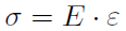
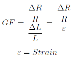
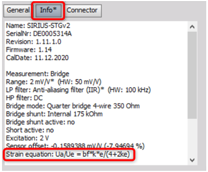
And now let’s prove the theory with real measurements with checking in the first step the mV/V reading. We first zero the sensor with “Balance Senor” (1) to read exactly the reading with performing “Shunt on” (2).

• The output value comes very close to the expected value (0,4995 mV/V).

Now let’s check the exact deviation of the strain result:

• We change the physical quantity to “Strain” and define the target value.
• After all the preparations are done, we perform the <Shunt Cal Check>

Image 63: Shunt calibration check

 The result of our shunt cal check looks very promising in this case (0,2 %). That means that the strain gage is OK.

Image 64: Result of shunt calibration

Notes about SHUNT CAL CHECK 

• We automatically compensate the sensor unbalance temporarily in the background to get the real signal deviation for the applied shunt. 
• The active strain gage must not get any load change (different strain) during the shunt calibration measurement. This additional sensor signal will falsify the result!

Shunt cal auto target:

If the shunt calibration target is not known or defined in the sensor database, we can automatically calculate the theoretic result based on the known strain gage and shunt resistor value. Let’s make e an example for a 350Ω strain gage resistor and 59.88 kΩ shunt resistor.

We see that the values in Dewesoft are corresponding to the formula above.

Image 65: Shunt cal auto target

• The value of \(R_{Shunt}\)  is automatically taken from the selected shunt resistor of the amplifier
• For the Quarter bridge, R is taken from the amplifier settings. For Full- and Half-bridge, the value must be entered manually. This entered value has no effect on the measured signal and is only used to calculate the target.
• The shunt cal target is calculated as the scaled sensor value (eg: µm/m, N or…)

Depending on the amplifier type, we offer different connection of the shunt. The selection below shows a connection to the shunt again Sns- which results in a negative signal and as well in a negative shunt cal target result.

Image 66: A negative shunt cal target result

Use custom shunt resistor: 
Many different values of shunt resistors are used from different suppliers.

• 59.88kΩ and 175kΩ for getting 1000µm/m at 120Ω or 350Ω (like on SIRIUS-STG type),
• 100kΩ like on most of all Dewesoft strain gage amplifiers,
• 320kΩ, 160kΩ, 80kΩ, 55kΩ and many others can be found as well on the market.

Sure, none strain gage amplifiers on the market can include all these different shunt values.
But how can we check the shunt cal target, the build-in shunt resistor of the amplifier does not match with the sensor data?

Let’s assume at 350Ω strain gage, where the shunt cal target \(T_{SNS}\) of 0.5 mV/V is defined with shunt resistor \(R_{SNS}\) of 175kΩ. We want to check this result with our SIRIUSi-HD-STGS module, where is the build-in shunt resistor  \(R_{AMP}\)  of 100kΩ.

We just need to enable the custom shunt to define the given value \(T_{SNS}\) of is defined for 175kΩ.

Image 67: Enable the custom shunt

With the <Shunt Cal Check> we have all information to calculate the deviation of the given result of the sensor with the formulas below.
The nominal target result for the amplifier \(T_{AmpNorm}\) would be:

But let’s say we are measuring \(T_{AMP}\)  with 0.8726 mV/V.
The nominal target result of the sensor \(T_{SNSNorm}\) would be:

The final indicated result will be:

Image 68: Indicated result

So independent of which shunt value defined in the sensor, we recalculate the result according to the selected shunt value of the amplifier.

In some cases, strain gages are mounted away from the measuring equipment. This distance increases the possibility of errors because of changes in temperature and lead desensitization. Therefore, lead-wire resistance changes. If we have a two-wire installation, that is shown in the picture below, two leads are in series with the strain gage and any change in the lead-wire resistance can't be distinguished from changes in the resistance of strain gage.

Image 69: Strain gages are mounted away from the measuring equipment

 
But this can be fixed. We can correct the lead-wire effect by adding an additional - third wire. This is shown in the next picture.

Image 70: Additional third wire

In this configuration, the third wire acts as a sense lead. No current is flowing through this wire. This option of wiring strain gages to a bridge cancels one part of the extension wire errors. If we look from the more theoretical side, if the lead wires, that run to the sensor, have the same nominal resistance, temperature coefficient, and temperature, full compensation exists. In real life, wires have a tolerance of about 10% and a three-wire installation doesn't eliminate the two-wire errors completely. But it sure reduces it. If the lead-wire resistance doesn't exceed the gage resistance and is small in comparison to it, that error isn't considerable. But if the lead-wire resistance exceeds 0.1% of the nominal gage resistance, this source of error becomes significant. Therefore, in industrial applications, lead-wire lengths should be minimized or eliminated by locating the transmitter directly at the sensor.

Lead wire compensation

As introduced above, the resistance of a lead wire is reducing the sensitivity of the strain gage signals due to the voltage drop. This reduces the voltage level on the active strain gage and therefore the sensitivity. The example below shows the reduction of 0.1Volt. The resulted sensitivity loss can be roughly

Image 71: Voltage drop and sensitivity loss 

This reduced sensitivity is also seen when performing shunt calibration. So we use shunt calibration to calculate \(R_{Leadwire}\) out of \(V_{S}\) , \(R_{Bridge}\) and \(R_{Shunt}\)

Out of the bridge resistance \(R_{Bridge}\) and the lead wire resistance \(R_{Leadwire}\) the compensation factor \(Corr_{Leadwire}\) is calculated:

With this factor, the raw data \(Data_{Raw}\) of strain gage amplifier is corrected to \(Data_{Corr}\). This corrected data is used for further processing inside the Dewesoft X software package: eg Sensor scaling, data storing, visualization...

With pressing <Compensate> in the channel setup screen all steps above are done in the back:

• Shunt calibration is initialized for getting Vs,
• \(R_{Leadwire}\) and \(Corr_{Leadwire}\)  are calculated and used for data further data processing,
• These values are stored together with the complete DewesoftX setup file.

Important note: the active strain gage must not get any load change (different strain) during the shunt calibration measurement. This additional sensor signal will falsify the result!

Below you can see the result for a 120Ω strain gage connection with a 100m cable of 0.25mm² to our amplifier. Without correction, the gain error would as high as 5.6% (!) and therefore significantly influence your measurement result.

Image 72: Strain gage connection result

After lead wire compensation, no additional Sensor balance is needed. The indicated Sensor unbalance (1mV/V) is shown correctly by rescaling with the above equation ( \(Data_{Corr}\) ).

Before compensation, this Sensor unbalance was shown as 0.944 mV/V to eliminate the sensor offset.

Image 73: Sensor unbalance

The lead wire compensation can be performed as well in Half-Bridge 3-wire or Full-Bridge 4-wire connection, where Exc and Sens are connected directly at the amplifier together.

Image 74: Exc and Sens connected together directly at the amplifier

At a different bridge and shunt configuration, the above formulas for getting \(R_{Leadwire}\) and \(Corr_{Leadwire}\) are different, but it follows the same principle.
For Full-Bridge 6wire, Half-Bridge 5-wire, or Quarter-Bridge 4-wire the lead wire compensation is automatically done by the amplifier. That’s why we don’t need any additional compensation settings.

Image 75: Automatic lead wire compensation result

 

 

We have several group operations (Channel actions). We can find them in the Channel setup.

Image 76: Channel actions

 

By pressing the three-dot button, we can add even more Channel actions. The amount of visible buttons depends on the functionality of the installed amplifier type. Dedicated functions for strain gage amplifier are only visible if installed.

Lead wire compensation

For activating the <Lead wire compensation> function for all channels, activate this button.

Image 77: DAQ actions

Now we can perform lead wire compensation for all installed channels in our system at once.

Image 78: Channel actions with Leadwire compensation

To see the result in the channel grid, right-click on the head line and select “Edit columns” and enable “Leadwire compensation. With this section, the result of each channel is shown in the channel table.

Image 79: Result of Leadwire compensation

 Shunt cal check

For getting a complete overview of the shunt call check result in the channel gird we have to enable Sensor check target", "Sensor check result", "Sensor check error" and "Group".

Image 80: Check the wanted result in the channel setup

 After performing the Shunt-Cal check, the complete result is shown in the channel table.

Image 81: Channel actions for Shunt-Cal check

 

Image 82: Multi-channel result for Shunt Cal check

Multi group actions

We can also make group operations with different groups. We do that by simply assigning one channel to "Group 1", and the other to "Group 2".

Image 83: Assigning different groups

 

Image 84: Group settings  


Now you can apply the channel operations group-wise.

Image 85: Applying operations groupwise

---

Example:
We will show the group operations in one short measurement.

For this experiment, we will use the Sirius instrument. We will start our measurement by connecting two tuning forks (quarter bridge, 3 wires, 350 ohms). Tuning forks can be connected to Sirius via STG adapters.

Unfortunately, the Sirius, that we are using, doesn't have two STG channels, so we will connect one tuning fork via STG and the second one via STG to MULTI converter. We already know how to set everything for 3 wire, 350-ohm quarter bridge connected via STG.

This is the setup:

Image 86: Setup for quarter bridge sensor

The settings are a bit different when it comes to the connection via STG to MULTI converter.

Let's take a look.

Image 87: Settings for the sensor connected to MULTI module

 We are able to choose Bridge measurement and bridge mode. But when we try to choose internal 175 kΩ bridge shunt value, this option isn't available. On this point, we need to explain one great feature of Dewesoft. Dewesoft recalculates all the values, no matter which bridge shunt you choose. That means, that the software automatically takes care if there are different resistor values. In the General Information tab, we have the 59.88 kΩ resistor present, but if we mark the Use custom shunt resistor, we can type in the correct value of the used resistor.

When entering the resistor value, the field gets yellow. We confirm the value by pressing <Enter>.

Image 88: Entering the resistor value

The software will then automatically recalculate the values, according to the given (Bridge shunt) and chosen resistance values. The asterisk (*) symbol after the result indicates that the check has been performed with a different resistor value than was physically available.

We can also perform group operations in Measure mode, so let's go there first. There we will see two new buttons: Zero and Amplifier. If the "Zero" button is not there, then sensors from the sensor database / TEDS sensors are most likely used, and changing the offset is not allowed. Check sensor settings in Channel setup or Sensor editor. If the ''Amplifier" button is not there, no amplifiers are set to "Used" in the channel setup.

Balance sensor

Balance sensor can be activated in the measurement mode only if storing is not active. Depending on the group settings in the setup screen, all channels can be balanced at once or only selected groups.

Image 89: Group operations in Measure mode

 

Shunt/Short at the beginning and end of the measurement

At the end of a measurement, you may want to check if the strain gage and the amplifier are still OK. You also want to see, if the bridge has drifted over time due to temperature or other effects.

Start the measurement and click the Store button. The "Zero" button will disappear, because zeroing also changes the channel min/max limits, and that is not allowed during measurement. Also, balancing the bridge is not possible at this state anymore. Do a "Short on for 1s", wait a little bit, then press "Shunt on for 1s".

Image 90: Shunt on for 1 second

 

 

Image 91: Shunt on for 1 second

 At the end of the measurement, when you are still storing do again a "Short on for 1s" followed by a "Shunt on for 1s". Stop the measurement and go to Analyse mode. Activate the cursors in the properties of the recorder instrument (on the left side).

Image 92: Time between the cursors

Move the white cursor I to the Short position at the start, and cursor II to the Short position at the end (grey arrows). You can also lock the cursors to not lose them when zooming in and out of a longer measurement.

The Delta will be shown on the right side. In our case, it is 0,0 measurement OK.

Image 93: Checking the time between cursors