Orbit analysis

Training course summary

In this course you will learn the basics of how to set-up and use Orbit analysis, and how to interpret the analysis results. 

The course will also include data examples and the main theory behind the calculations, and in the end you should have gathered enough information to be able to get started using the application yourself. 

As for all DEWESoft courses, this course is completed with a quiz. The quiz will have questions for which the answers can be found in the course material.     

Why should you use Orbit Analysis?

Steady, continuous operation with as few malfunctions and vibrations as possible is essential for maximizing productivity and ensuring the reliable operation of a machine - whether a huge rotating mass in a power plant or a high-revving compressor. Knowing the rotor movement, then different phenomena of lubrication and bearing states can be determined and consequently, machine operations can be optimized.

To achieve this, measurement and analysis of rotational vibration data is crucial. Dewesoft Orbit analysis is an ideal analysis tool for rotor dynamic movement examination, assessment of any motion restrictions causing vibration, and consequent prevention of potential, unwanted damages to rotating machinery that would result in premature wear of components and could cause critical failure.

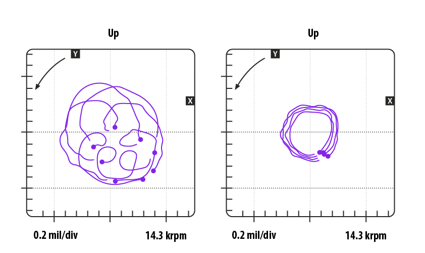
Orbit analysis can monitor and analyze the current state of journal bearings and how such bearings have behaved over time while in operation. 

Orbit analysis is designed specifically for such bearing types to inspect and diagnose shaft / journal movement, the oil lubrication, and the clearance.

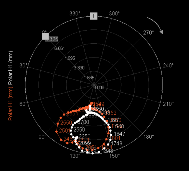
Dedicated display widgets for orbit analysis helps create a clear overview of the state of one or multiple bearings. Such analysis is crucial to understand the impact of the lubrication oil, the shaft load, the rotation speed, the clearance, and the wear and tear of bearing. 

When should you use Orbit Analysis?

Orbit analysis is applicable for analysis of journal bearings. Journal bearings are also sometimes referred to as bushings, plain bearings, or sleeve bearings. These bearing types all have a fluid lubrication layer in between the shaft and bearing which makes the shaft have a sliding action with a loose movement within the clearance.  

Orbit analysis is not applicable for roller bearings and gears, or other bearing types having roller action or direct connection between the shaft and bearing, since you do not have a fluid medium / lubrication in between, and hereby no loose shaft movement. Instead, for such direct contact bearings and gears Order analysis is the proper application.

What is needed to configure and get going with Orbit Analysis?

The basic measurement setup for orbit analysis consists of: 

• pair of proximity probes (also called eddy-current probes) per bearing, 
• a keyphasor (3rd proximity probe or a tacho sensor), 
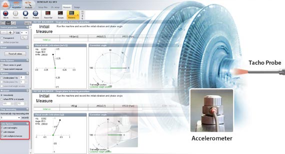
• a data acquisition system, 
• orbit analysis software, 
• and a computer.

By detecting the shaft proximity in two directions (x and y) rotor movement is calculated and displayed throughout the measurement.

Dewesoft Orbit Analysis system is very flexible and can be configured for single or multiple bearing measurements at the same time. The input channel count can be expanded at any time. DAQ system can also be configured to allow different sensor connections at the same time - thermocouples, RTDs, IEPE/ICP® accelerometers, strain gauges, and more.

The typical Orbit analysis measurement system will consist typically of the following elements:

• SIRIUSi isolated data acquisition system with 8xLV signal amplifiers or 6xLV-2xLV+ (additional two counter) amplifiers.
• 2-8x Eddy-current probes
• DewesoftX Orbit Analysis option

Optional:

• FFT Analyzer option
• Order tracking analysis option
• Rotor balancing option
• OPC UA Client/Server option
• Historian time-series database
• MODBUS protocol option

Orbit analysis is one of the main diagnostics tools for rotating machinery using journal bearings, such as turbomachinery. Turbomachinery provides kinetic energy to operations enabling movement - a function that is widely used in industrial processes to move solids, liquids, or gases through drivers, driven components, and transmissions such as:

• Compressors
• Drills
• Generators
• Turbines
• Engines
• Pumps
• Blowers

Such rotating machinery as shown above is applied in a variety of industries, e.g. automotive, chemical, oil and gas, metals, HVAC or mining, and in the majority of different power plants:

• Hydroelectric
• Nuclear
• Thermal
• Gas
• Coal
• Biomass

Below is an example that shows how a journal bearing is monitored at a hydropower plant. By monitoring the shaft centerline position together with both orbit plots, polar plots, shaft speed, and much more, it is possible for the operator to follow the bearing condition, both regarding bearing wear and tear, but also regarding e.g. lubrication oil conditions. 

A proximity sensor is able to detect a nearby object without making contact with it, and then output a pulse or voltage signal. There are several types of proximity sensors, which are chosen based on the composition of the object(s) that should be detected. 

For example, an inductive proximity sensor creates an electromagnetic field around its measuring end. According to the well-known magneto-resistive effect, the resistance of certain objects (particularly ferrous ones) will change when they are exposed to magnetic fields. Most proximity sensors take advantage of this effect by creating a small magnetic field and then detecting when it is interrupted or changed significantly due to the presence of such material. 

So when we place such a sensor near a rotating shaft and then affix a ferrous feature onto the shaft that will pass close to the sensor with each revolution, we have a very reliable and accurate speed sensor. The sensor detects the field interruption and outputs a pulse or voltage signal that any DAQ system can display and record. 

There are also capacitive proximity sensors that can detect non-metallic objects, using the principle of capacitive coupling. Instead of an electromagnetic field, they generate an electrostatic field. As an object enters this field it changes the capacitance in the sensor’s oscillator circuit. This is detected by the sensor which then creates an output. In the case of both magnetic and capacitive proximity sensors, their sensitivity to the target object can be adjusted. 

Proximity sensor pros:

• Very reliable because they never make contact with the objects being detected. Wear and tear are virtually non-existent

• Very low initial and operating cost

• Capacitive types can also be used to measure the thickness

• Inductive types are not affected by water, mud, etc.

Proximity sensor cons

• Limited detection distances - most inductive sensors are limited to 70mm (2.76 in.)

• They require external power

In the Analog in setup, the channels need to be configured for use of proximity probes.

 Most often the configuration per bearing consists of three eddy-current probes: Y, X and Keyphasor. 

Depending on whether the utilized eddy-current probes use a separate signal conditioner or are connected directly to the input on Dewesoft HW, different amplifiers are used. 

For both cases, Voltage mode is selected under Measurement and Displacement/distance as a Physical quantity.

The Orbit analysis module can be added to a setup by clicking on the “+ More” button where various application modules are available.

When adding the module the following module setup appears: 

• Frequency channel setup
• RPM setup
• Calculation setup
• Runout compensation
• Reference orbit
• Machine configuration

Frequency channel setup

To determine the engine rotation speed, a source of frequency needs to be configured. For Orbit analysis, a third proximity probe also called a keyphasor is most often used as it detects a flat or wedged section on the shaft and this generates the needed pulse per revolution from which operating speed is concluded. 

To allow different configuration possibilities to the user, the Orbit Analysis module supports several different sensor types to be selected as the frequency source:

Counters

For Orbit Analysis several pulses or transient spikes per revolution are often used, meaning Tacho (digital) would be used for such application when it comes to sensors that are connected and configured as counters.

For multiple configuration possibilities, a variety of additional counter sensors are available in the dropdown: multiple Encoders as well as CDM sensors. In addition, different filter settings can be applied to selected frequency source signals.

Counter math

With the Counter math module it is possible to determine and recalculate counter angle- and frequency outputs while measuring, online, and during datafile analysis after a measurement, offline. 

This can be useful when you e.g. want to fix a faulty counter setting that wasn’t caught during the measurement, or if you want to tune a setting or two to see if that produces better results.

Counter math supports features like frequency smoothing, teeth size adjustment, software filters, and angle wrapping.

If the results from Counter math turn out to be better for your specific data file, you can also use the math output as input to other modules that work with counters, such as Orbit analysis, Order Tracking or Torsional Vibration.

Analog pulses

When having the Frequency source set to Analog pulses an analog time channel must be selected (different sensors generating analog pulses are supported).

• Tacho(Analog): 1 pulse per revolution using a proximity probe or a similar type of analog sensor 
• 36-2 (Analog) or 60-2 (Analog): sensor with 58 or 34 teeth and two missing teeth 

To configure the selected Analog sensor, click on the three-dot icon to open the Angle sensor math setup.

In the Angle sensor math setup, additional settings are available to configure the sensor:

• Trigger edge
• Trigger level (can also be found automatically by selecting ‘’Find’’), 
• Retrigger level, 
• Retrigger time, 
• Output channel unit (Hz or RPM) and 
• Averaging 
• a preview of analog tacho signals and triggers. 

The Lowest detectable frequency limit is definable in the user input field - the system will not detect frequencies lower than the specified value.

RPM channel

 Besides analog and digital sensors, any signal or channel directly representing the RPM (e.g. 0-10V equals 0-4500 rpm) can be used as a frequency source. As this option does not contain zero-angle information the extraction of phase is not possible. 

Under the RPM setup section, Lower and Upper RPM limits are defined as well as Delta RPM width and the direction of the test.

To configure the analysis according to the test conditions of the particular rotating machinery during the measurement and to get all of the needed data RPM setup section includes the necessary settings that apply to the direction, speed range of operation as well as the density of calculation of values during the test run. 

Direction

Orbit analysis supports the measurement of different machine operation scenarios: whether only the runup, coastdown, or both need to be measured, the analysis is easily configured accordingly via a dedicated dropdown. 

As turbomachinery often runs for long periods in steady state conditions between the runup and coastdown, selecting Both in the dropdown will automatically create a third operating condition as well: Steady-state. Each Direction creates a dedicated set of channels for the display of measured data so they can be displayed on separate widgets or all together on the same one for comparison.

Delta RPM

Delta RPM defines the change of speed at which data is updated during the measurement for the speed channel and all Orbit Analysis output channels containing speed information: Filtered orbit(e.g. Orbit H1), Shaft centerline, Polar plot, Order Waterfall vs. RPM and FFT waterfall vs. RPM

Lower and upper RPM limits

Upper and Lower RPM limits define the range for calculation and are used to correctly set up the resampling algorithm, depending on the max order extracted. They should be set by the expected speed range of the machine being measured:

Direction control

This makes it possible to control the Direction under Measure for multiple Orbit Analysis modules at the same time. In setups with multiple added Orbit Analysis modules and at the same time using the Direction Both, you can select to link the Direction control together instead of having to change the Direction for each module individually. 

The Mode parameter can be set to Master or Client. For Clients, you must select which Master it should be linked to. 

For example, if module OA1 is Master and module OA2 is a client to OA1, then this two modules are linked and Direction changes under Measure for one of them will also apply the same change to the other one:

Harmonic list

The extraction of desired filtered orbits is configured by inputting the order numbers in the harmonic list field, separating the entries in the list with a semicolon (;). In the below example, the first, second, and third harmonic orbits are extracted.

Order resolution

Selected order resolution defines the steps on the order waterfall between individual extracted orders. The higher the resolution the higher the number of lines between the orders.

Maximum order to analyze

Depending on the measurement application, the maximum order to analyze needs to be set high enough to still capture all the wanted orders. If, for example, a higher number of orders are not needed in the analysis, a lower value can be selected from the dropdown to consequently lower the needed sample rate and the amount of data stored. 

Time FFT lines

Affects the FFT cascade output, a higher number of lines results in better resolution and higher CPU load (supports Auto, predefined values selection from dropdown or arbitrary definition of a number of lines. )

Bin update

Bin update is used to define how the output data for each RPM speed bin is calculated.

• Always - When multiple values or spectra belong to the same bin, then the newest bin values will overwrite previous values and the newest values will be used in the output for that bin.
• First time - When multiple values or spectra belong to the same bin, then only the first bin values will be used in the output for that bin.
• Average - When multiple values or spectra belong to the same bin, then averaging for the values and individual and spectral lines will be performed over all values belonging to that bin.
• Maximum - When multiple values or spectra belong to the same bin, then the maximum value for all values and individual spectral lines across all spectra belonging to that bin will be kept.

FFT window

Different windows are available for the FFT:

• Rectangular, 
• Hanning, 
• Hamming, 
• Flat top, 
• Triangle, 
• Blackman (selected by default), 
• Exponential down and 
• Blackman - Harris. 

Amplitude

Depending on the selected amplitude in the dropdown, the following scaling is applied to the Bode plot and Polar plot: Peak, RMS, Peak-peak

Frequency axis unit

Frequency axis unit for FFT waterfall vs. RPM can be selected from the dropdown list.

Separate spectra per direction

Separate spectra per direction will create the selected spectral channels under all Directions channel groups. When disabled the spectral results will be combined across all directions.

Update interval

Update interval defines the criteria on which data, such as speed, shaft centerline and polar will be updated during the measurement.

There are two different criteria for update of data: 

• On RPM change (Delta RPM) - data is updated each time a defined Delta RPM value is exceeded. This is usually selected if the measurement consists of runup or coastdown or both. 
• On time - Values are updated on a defined time interval, regardless of the Delta RPM specified. This update criterion is suitable for steady-state operating conditions when RPM change criteria are not going to be triggered. Both update criteria can be selected at the same time to appropriately cover different operating conditions.  

Orbit analysis waterfalls

The Orbit Analysis module supports Order waterfall spectrograms vs. RPM and vs time, and at the same time FFT waterfall vs, RPM. 

They are enabled easily by ticking the checkbox in the Ch. setup section. They are shown using the 3D Graph widget which is further explained in the Measurement & Visualisation section

Vs. RPM spectra can be created both as Single-sided or Two-sided spectra. Single-sided spectra will have an order or frequency axis starting from 0. Two-sided spectra will have an order or frequency axis centered around 0. 

Two-sided spectra can be of interest when analyzing the phase difference between the X and Y-bearing sensors. 

Overall vs. RPM

Overall vs. RPM, results are 2D arrays with overall displacement levels across the defined RPM speed range. Such results can be a good way to overview and document critical speed intervals which should be avoided.

Runout compensation is performed to remove shaft irregularities from the measured values during the analysis. In the Ch. setup, the desired speed RPM at which the compensation is going to be performed is defined by the user, as well as the number of Averages (revolutions) to be taken into the calculation and the desired angle Resolution. 

Under Measure, the Orbit analysis module provides a display template design for the runout compensation measurement. When the runout Start button is pressed the runout measurement will start and the number of Averages will begin to count up.

The Runout compensation values are calculated in the angle-domain. This means that you can perform runout compensation measurements while running with variable speeds.

Reference orbit is a great tool for easy comparison of current operating conditions to those from a previous measurement. 

During the measurement, reference orbit can be easily acquired through a dedicated measurement screen.

The number of averages taken into the measurement is defined by the user in the Averages field. 

• Averages - specifies how many times the deflections at individual angles are averaged together.
• Lockable cursor calculation - Used when calculating runout compensations and reference orbits in Analyze mode (post-processing). Set this parameter to the desired calculation type to use the correct lockable cursors.

After measuring reference orbits the determined values can be illustrated under the Bearing Setup section after pressing the Paste button. The data will be added to the selected reference orbit table:

Any number of bearings can be defined with Dewesoft OA into the machine train. Machine configuration setup can be further broken down into subsections:

1. 1 - Quick settings
2. 2 - DC gap
3. 3 - Bearing setup

Quick settings

Under the Channel, the right input channels need to be assigned as probes X and Y for the individual bearing. 

Next, the angles and positions at which the probes are mounted need to be configured.

To make the configuration of the Angle and position easier, the graphical representation is available upon entering the Bearing setup

DC gap

Most of the time when proximity probes are mounted, there will be a certain DC component present. Dewesoft Orbit Analysis supports easy measurement of the DC gap by clicking on the Measure button next to the individual probe. 

After the DC gap is measured, a value will be shown in the DC Gap column. DC Gap can also be input manually in the Bearing setup window as explained in the next section.

Bearing setup

Upon selecting Setup under Machine configuration, a dedicated Bearing Setup window is opened, containing all of the advanced settings for configuration of the bearing settings:

• sensor configuration, 
• subsynchronous orbit extraction, 
• shaft and clearance circle configuration, 
• average orbit definition, and 
• DC gap manual input.

Inside this setup window, the user defines the runout compensation as well as the reference orbit.

Bearing properties

Under the Bearing name, a unique name can be input by the user to easily recognize which component it corresponds to.

Sensor

The graphical representation of the shaft together with direction and angle helps with the correct configuration of the sensor settings. 

In this section, the user selects the configuration: 

• Pair is selected when two probes per bearing are used and 
• Mono in case only one is used.

Besides selecting the configuration, the right probe channels need to be assigned to Y and X positions as well and their angle and direction need to be set. 

The same needs to be done for the Keyphasor under the Tacho angle.

Dewesoft Orbit Analysis supports extraction of subsynchronous orbit which can be used to detect fluid-induced instabilities such as whirl & whip. The calculation of the subsynchronous orbit is enabled via a dedicated checkbox and tracking filter bandwidth is defined in the corresponding input field:

Runout compensation

Runout compensation is necessary whenever shaft irregularities in shape are present which could be misinterpreted as movement during the measurement. Dewesoft OA supports multiple ways of establishing the runout compensation: 

1.) Paste - allows the user to paste values for runout compensation from previous measurements. The angle step needs to be defined the same in the Ch. setup as it was for the data that will be pasted and the data structure of the columns needs to be as stated below in the Import paragraph. 

2.) Import - allows import of .txt files containing the runout compensation data. The data structure is important as it needs to contain an angle in the first column, a Y value in the second, and X in the third. A good way to achieve correct structure is to input it in separate columns in Microsoft Excel and then save it as a .txt file. Example .txt file is seen below: 

3.) Measure - The last and perhaps most important way of determining the runout compensation is to measure it directly with Dewesoft. This is also the easiest way of doing it as it requires a single click operation in Measure and calculated values are automatically stored in the Ch. setup.

 Shaft

This section of channel setup is dedicated to the configuration of shaft-related settings. The direction of shaft rotation is selected in the Rotation dropdown. The drop-down allows the user to select between CW - clockwise direction and CCW - counterclockwise direction.

The Position dropdown defines the starting position of the shaft regarding the diameter of the bearing.

Clearance

Dewesoft Orbit Analysis supports a straightforward definition of the clearance circle under the Clearance section of the Machine Configuration Setup.

Users can select between Circle and Ellipse shapes for the clearance circle and use the input field to input the clearance circle Radius (circle) or Width & Height (ellipse).

Average orbit 

The average orbit can be configured to show more than a single revolution at once. This is defined by the input value in the field Periods - 5 periods means the average orbit will show 5 revolutions. 

The user also defines the number of averages to take into the calculation of the average orbit by inputting the desired number into the Averages input field.

DC gap

Besides measuring and automatically compensating for the DC gap, Dewesoft Orbit Analysis allows the user to manually input the DC gap values. 

This is especially useful with large turbines as seen in power plants where completely static conditions with 0 RPM are rarely seen. In such cases, the DC gap was measured upon mounting the probes and is manually input for later measurements.

• Monitoring and alarms

• Data output streaming to 3rd party system

• Report generation

In total, the Orbit analysis module contains many different result types of which many of the types will generate multiple channel results. The full list of output results from the Orbit analysis module, including a small description, of how many of such types will be created, and which display widgets to use for illustration, are all listed in the table below:

Each bearing with assigned channels added to the machine train will automatically create a dedicated pre-defined display. On the predefined display, there will be a set of Orbit plots, Polar plots, and 2D graphs as well as a Digital meter for speed and an Input control dropdown to select between different operating conditions if Both are selected under RPM setup.

Orbit plot

The Orbit plot is a specific widget for the Orbit Analysis module. The plot shows data from two time domain channels, plotting a two-dimensional visual picture of the motion of a rotating shaft. 

The widget shows graphically the position of the proximity probes together with the tacho (keyphasor) position and direction of rotation.

There are different output channels available in the Orbit Analysis module that can be shown on the Orbit plot:

• Raw orbit,
• Average orbit,
• Filtered orbit (e.g. Orbit H1, Orbit H1, …),
• Subsynchronous orbit and
• Shaft centerline

When the Orbit Plot widget is selected, on the left side of the Measure display a tab of settings is available for the configuration of the axis to the user: 

Number of ticks - changing the number of ticks will increase them on the Orbit plot accordingly. The left picture below shows 5 ticks and the right picture shows 15 ticks: 

Auto scale - ticking the checkbox will automatically scale the axes of the Orbit plot. There are two different Auto scale types: Absolute and Relative. 

• Absolute auto-scale always keeps the zero in the center of the plot and therefore gives a better indication of orbit size and position relative to the center of the bearing: 

• Relative auto-scale sizes the axes according to the maximum current dimension of the measured orbit. This makes the orbit shape easier to observe and acts as a sort of zoom. The zero in this case is not always in the center position: 

Single axis - this checkbox determines the behavior of how channel names are shown next to the orbit plot when showing multiple channels on the same graph. In the below example, two harmonic orbits are shown on the same orbit plot. The left image shows a single axis switched on and the right image shows a single axis switched off: 

Besides axis configuration, there are different Drawing Options available when the Orbit plot widget is selected: 

Graph type - The user can select either Grid or Circle. The difference between the two graph types is shown below - the left image shows a Grid and the right image shows a Circle: 

Display type - The user has the option to select either RPM or Time (in seconds) to be displayed when the Shaft center is assigned to the Orbit plot. The below images show the difference, the left image displays RPM and the right image displays Time together with the shaft center points: 

Raw orbit, also called Direct orbit, directly plots scaled time-domain data from a pair of orthogonal probes mounted at the same axial position on the rotating machine.

Raw orbit channel group can be displayed on the Orbit plot .

The 2D graph widget supports multi-trace and multigraph display of data meaning the average orbit can be shown both ways on the 2D graph. 

Average orbits from different bearings can be displayed on the Orbit Plot in multigraph mode.

 Average orbits from two bearings positioned closely along the shaft length displayed in multi-graph mode on Orbit Plot:

Average orbits from two bearings positioned closely along the shaft length displayed in multi-trace mode on 2D graph:

Average orbits from two bearings positioned closely along the shaft length displayed in multi-graph mode on 2D graph:

Filtered orbit, also called harmonic orbit, represents the extracted orbit of the order that has been input by the user in the Harmonic list section of the Calculation setup. 

For each harmonic entered into the harmonic list, a separate channel is created:

Each created Filtered orbit channel data can be displayed on the Orbit Plot widget. As with Raw orbit and Average orbit, the Filtered orbit can be shown in multi-trace and multigraph modes.

Filtered orbits H1-H4 displayed in multi-trace mode on Orbit plot:

Filtered orbits H1-H4 displayed in multi-graph mode on Orbit plot:

Polar plot is a dedicated widget, featured in the Dewesoft Orbit Analysis module. It allows representation of Amplitude, Phase and Speed together with the shaft center on the same display for a comprehensive, single widget overview of the machine operation. 

Each probe has a set of dedicated, corresponding polar plots for each order of extracted filtered/harmonic orbit. The polar plots for runup, coastdown and steady state are written into separate channels, depending on the selection of the dropdown Input control, Output channels and visual representation. 

The predefined Orbit analysis measurement display comes with a Polar plot widget for each of the used probes per bearing. When using OA with a pair of probes this means a pair of Polar plots is autogenerated and each one represents data from one of the probes - Y and X.

The Orbit waveform graph widget plots bearing X and Y sensor displacement data across a user-defined time duration or across a specific number of revolutions. 

Each new tacho key phaser crossing is indicated with a dot in the graph as illustrated below:

When a fixed time duration is selected, then the number of revolutions varies as time goes on, as illustrated above. 

A fixed time duration can be selected by setting the History type parameter to Time. You can determine the time duration (Display time) shown in the graph.

If the History type is set to Revolutions then you can select the number of Revolutions you want plotted. 

With the History type set to Revolutions, you also have the option to either have an axis with a fixed Revolution count or Angle, or to have a variating Time length on the axis that changes as the revolution speed changes, such that the number of plotted revolutions are kept constant.

Throughout the years of Orbit Analysis evolution, there was a set of display layout designs developed that are typical for the application. As Dewesoft offers advanced customization possibilities it is easy to create, edit, and transform the typical display layouts within a few clicks. In the following sections, you will find examples of how to generate such display layout templates.

Raw orbit with clearance circle

Created by assigning the Raw Orbit channel group to the Orbit Plot widget and switching the clearance circle option on the left side widget settings. Clearance circle needs to be defined beforehand in the Orbit Analysis channel setup.

Full motion graph

Created from Raw orbit with Clearance circle by adding the Shaft center channel to the Orbit plot. In other words, it is created by assigning the Raw orbit and Shaft center to the Polar plot widget and switching on the Clearance circle. Clearance circle needs to be defined beforehand in the Orbit Analysis channel setup.

Runout compensation, sometimes called slow-roll compensation, is applied to compensate for any shaft irregularities (flattenings or other variations in diameter along the circumference variations) that would have otherwise been picked up by the proximity probes together with the actual movement of the shaft.

The compensation is typically performed at low rotational speeds when the shaft is rotating slow enough for it to remain stationary (in regards to the movement inside the bearing clearance). However, not all rotating machinery is the same and some of the machines require compensation to be performed at higher speeds.

To cover all different runout compensation scenarios, DEWESoft Orbit Analysis performs such measurements in the angle domain which equals variable speeds, and allows users to determine the angle resolution and number of rotations to be averaged into the compensation.

After it has been set up in the Ch. setup, the compensation itself is performed through a dedicated measurement display, that is generated automatically together with predefined Overviews for each Bearing and and a Reference Orbit display.

The predefined Runout compensation display consists of the following elements:

1. 1. Recorder with raw signals from proximity probes
2. 2. Start button to initiate the runout compensation
3. 3. Measurement status
4. 4. Current speed of the machine

Upon starting the measurement, the status in the measurement status bar switches from Ready to displaying the measurement progress. The measurement itself takes the number of averages that were user-defined in the Ch. setup section under Runout compensation.

The system displays the status Done after the measurement of runout compensation has been completed successfully:

After the Runout compensation measurement is Done,, the calculated values are automatically added to the setup and can be seen under Ch. setup under the Machine configuration - Bearing Setup page:

In case the Runout compensation display needs to be manually added, this is done through the following steps:

1. 1. Select Displays
2. 2. Select + the button
3. 3. (Optionally) Go to the Add sub-display tab
4. 4. Select Runout compensation

Orbit analysis can be recalculated using the raw signals from the proximity probes and the frequency source that has been stored during the measurement. To recalculate data simply open the datafile with the raw signals included and in Analyze mode navigate to Offline math:

1. When in Setup, add the Orbit Analysis by selecting More… and choosing Orbit Analysis from the list of modules:

2. Having added the Orbit Analysis module, configure it by following the same steps described in the previous sections.

3. Return to Review and select Recalculate

4. The recalculated output channels are now displayed on the predefined display.

Recalculating Runout correction

Together with all of the output channels from Orbit Analysis, Runout compensation can also be recalculated in post-processing using the raw data from the proximity probes.

To recalculate and apply runout compensation in Analyze mode, please follow the steps below:

1. Navigate to the Runout compensation sub-display template.

2. In the Runout compensation display, place the two cursors over the section of raw data you wish to use for the runout compensation and lock them.

3. Click on Recalculate to determine the runout compensation data:

If you see an Offline math button instead of the Recalculate button then set the Orbit analysis module to Offline first under Setup.

4. After Recalculation, the calculated values are automatically added to the setup and can be seen under the Machine configuration - Bearing Setup page:

Recalculating reference orbit

From acquired raw data it is possible to define the reference orbit also in Analyze mode. To recalculate and store the reference orbit in Analyze mode, please follow the below steps:

1. Navigate to the pre-defined Reference orbit sub-display template:

2. Place the two cursors over the desired region from which you wish to acquire data to define the Reference orbit, and then lock the cursors:

3. Select Recalculate. If you see an Offline math button instead of the Recalculate button then set the Orbit analysis module to Offline first under Setup.

4. Now the newly calculated Reference orbit data are copied to the clipboard and can be pasted directly into a Reference orbit data table found under the Bearing Setup page.

Normal operation is indicated by acceptable vibration at all measurement positions. Critical speeds may be excited during speed transients, but the amplitude will be acceptable. Trend plots show constant amplitude with little or no variation with load. The dominant vibration frequency is 1X with little or no vibration at any other frequencies.

Amplitude trend

The amplitude trend plot indicates constant amplitude with no significant load or time dependency.

1X phase trend

1X phase trend will show a constant phase value over time.

Waveform

Direct waveform plots show no truncation, frequencies other than 1X, or spikes.

Spectrum

The half-spectrum plot shows one dominant peak at 1X frequency with no significant vibration at other frequencies.

Full spectrum

The full spectrum plot shows one dominant positive peak at +1x frequency with no significant vibration at other frequencies. Peak at -1X is lower than +1X.

Direct orbit

Circular or slightly elliptical orbit with no evidence of truncation or loops. Phase trigger indicates forward precession.

Shaft centerline

The shaft centerline plot shows the normal path from zero to full speed with no sudden changes. Eccentricity remains below the vertical centerline at full speed.

Bode plot amplitude

The bode plot (amplitude) shows acceptable amplitude at a critical speed. Some variation between startup and coastdown responses is typical.

Bode plot - phase

The bode plot (phase) shows a smooth phase shift through typical speed, with the rate of change matching previous runup or coastdown events. The phase at full speed and very low speed is consistent between events.

Polar plot

The polar plot shows similar amplitude at low speed, through critical speed, and at full speed between transient events with acceptable maximum amplitude at critical speed and at full speed.

Waterfall

The waterfall plot will show fairly constant amplitude through multiple periods with no significant variation in the 1X amplitude.

Other operational symptoms

Bearing temperature trends are constant with speed and load and below alarm limits. The audible noise near the machine does not indicate any changes from previous surveys or any abnormal rattling.

A sudden imbalance may be caused by a blade loss, loss of balance weight, or another component normally attached to the rotor. This may occur during normal operation or a load or speed transient. It can be differentiated from an electrically induced imbalance because the changes in vibration characteristics (amplitude/phase) are not reversible by changing load or speed.

Amplitude trend

Vibration amplitude trends show a sudden increase in amplitude. Similar step changes may be noted in vibration phase trends.

1X phase trend

1X phase trend will show a step change. The phase may increase or decrease depending on the angle between the location of the lost material and the residual unbalanced vector.

Waveform

The direct waveform plot (at the time of damage) will show a sudden increase in amplitude. If the amplitude is excessive, some truncation may be present.

Spectrum

After the event, the half spectrum will show an increase n 1X amplitude compared to before the event. Some small-amplitude peaks at n-X frequencies may be present.

Full spectrum

The full spectrum plot will show an increase in both +1X and -1X peaks. There may be some increase at +/- n-X frequencies. The +1X will be higher than the -1X peak unless another fault is present.

Direct orbit

Direct orbit plot will show an increase in amplitude as well as a phase change before and after the event indicated by a change in the position of the phase trigger marker.

Shaft centerline

The shaft centerline plot will normally show a jump in position immediately after the event, and the shaft will return to near the pre-event position shortly after.

Bode plot - amplitude

The bode plot (amplitude) will show an increase in amplitude at all speeds after a blade loss. Critical speed will not change, and the amplification factor should be approximately the same as before the event.

Bode plot - phase

The bode plot (phase) will show a constant phase shift from before and after the event that is constant at all speeds.

Polar plot

The polar plot shows an amplitude increase and a phase shift after the event. The phase shift will be constant at all speeds.

Waterfall

The waterfall plot will show a step change in the 1X amplitude after the event occurs.

Other operational symptoms

The increase in vibration amplitude caused by sudden unbalance may result in an increase in bearing metal temperature. If the lost component becomes lodged in the turbine, the noise may increase as indicated by rattling or broadband noise due to flow disturbances.

Misalignment will generally result in elevated vibration amplitude due to load transfer from one bearing to an adjacent bearing. The increase will show up as higher amplitude at 1X and 2X in spectrum plots, with 2X amplitude reaching or exceeding 1X amplitude as the severity of the misalignment increases. The misalignment may be coupling or internal misalignment caused by improper bearing elevations.

Amplitude trend

Vibration amplitude trend plots will show increased amplitude in the presence of excessive misalignment.

1X phase trend

1X phase trend will generally be unaffected by misalignment.

Waveform

Misalignment will often result in a 2X response. This will be apparent in the direct waveform plot with an increase in peak-to-peak amplitude and 2X frequency component.

Spectrum

The half-spectrum plot will show elevated 2X vibration in the presence of misalignment. The relative amplitude of the 1X and 2X peaks is indicative of the severity of the misalignment.

Full spectrum

The full spectrum plot will show an increase in the +/- 1X and +/- 2X peaks. The positive peaks will generally be higher than the negative peaks.

Direct orbit

Direct orbit plot will show evidence of the constrained shaft motion from the misalignment. More severe misalignment may result in an orbit resembling a banana or even a figure-eight shape.

Shaft centerline

Misalignment may result in a shaft centerline plot that shows the rotor position farther away from the bearing center. This would be dependent on the severity of the misalignment. 

Bode plot - amplitude

An amplitude bode plot will generally be unaffected by misalignment, other than an increase in amplitude at all speeds over a properly aligned machine.

Bode plot - phase

The phase of the bode plot will be unaffected by misalignment.

Polar plot

A polar plot will generally be unaffected by the misalignment other than an increase in amplitude at all speeds over a properly aligned machine.

Waterfall

Waterfall plot vs. time will show elevated 1X and 2X vibration in the presence of misalignment. The relative amplitude of the 1X and 2X peaks is indicative of the severity of the misalignment.

Other operational symptoms

Elevated bearing metal temperatures, combined with higher 1X and 2X orders of vibration can be a strong indicator of misalignment. The elevated bearing temperature may be caused by both the higher vibration amplitude and the increased static load reacted by the bearing in the presence of misalignment. 

Oil whirl is normally caused by improper design of the rotor-bearing system. The presence of vibration components at frequencies slightly less than 1/2X with varying amplitude are indications of oil whirl. Oil whirl can be aggravated by higher speed, higher oil viscosity, and lighter bearing loading.

Amplitude trend

The overall amplitude trend will normally show a high average amplitude with large variations in the presence of oil whirl.

1X phase trend

The 1X phase trend will generally be stable with constant speed in the presence of the oil whirl.

Waveform

The time waveform plot will show both 1X vibration and a subsynchronous component near 0.48X with an amplitude that varies over time

Spectrum

The half spectrum will show a 1X peak and a peak slightly below 1/2X that will normally vary in amplitude over time.

Full spectrum

The full spectrum plot will show forward precession and a subsynchronous peak at slightly less than 1/2X.

Direct orbit

The direct orbit plot will show the 1X and the slightly less than 1/2X components. The phase marker will slowly shift in the direction opposite rotation, but the vibration precession will remain forward.

Shaft centerline

The shaft centerline position will generally be unaffected by the oil whirl, however, operation near the bearing centerline will be more susceptible to oil shirl

Bode plot - amplitude

The amplitude plot will generally be unaffected by the oil whirl.

Bode plot - phase

The phase will generally be unaffected by the oil whirl.

Polar plot

Polar plot will generally be unaffected by the oil whirl.

Waterfall

A cascade plot will show the onset of instability with a subsynchronous peak showing up at a frequency slightly less than 1/2X.

Other operational symptoms

Oil whirl vibration may be affected by changing the lube oil supply temperature. This has the effect of changing the rotor dynamic coefficients of the bearing. These changes have a limited impact on whirl vibration.

Oil Whirl will transition to Oil Whip when the whirl frequency reaches the first natural frequency. 

The sub-synchronous vibration will lock onto the unstable natural frequency and will not continue to increase with the rotor speed. The sub-synchronous vibration will increase and can be damaging.

Amplitude trend

The overall amplitude trend will show very high amplitude in the presence of a whip. The amplitude may increase until a limit cycle is reached.

1X phase trend

The 1X phase trend will generally be stable with constant speed in the presence of the oil whip.

Waveform

The time waveform plot will show both 1X vibration and a subsynchronous component at the unstable natural frequency.

Spectrum

The half spectrum will show elevated 1X and very high subsynchronous vibration at the unstable natural frequency.

Full spectrum

The full spectrum plot will show elevated +/- 1X and very high subsynchronous vibration at the unstable natural frequency.

Direct orbit

The amplitude in the direct orbit will grow after the transition from whirl to whip. The precession will remain forward, and the phase marker will continuously shift in the direction opposite rotation at a faster rate.

Shaft centerline

The shaft centerline position will normally be unaffected by oil whip except that operation near the bearing centerline will be more susceptible to oil whirl.

Bode plot - amplitude

A bode plot - amplitude, will generally be unaffected by oil whip.

Bode plot - phase

A bode plot - phase will generally be unaffected by oil whip.

Polar plot

A polar plot will generally be unaffected by oil whip.

Waterfall

A waterfall plot will appear similar to an oil whirl until the transition to whip. The subsynchronous vibration frequency will remain constant.

Other operational symptoms

Oil ship will be extremely destructive to the turbine generator. The vibration amplitude will generally grow over time.

Operating a turbine generator on a critical speed or a structural resonance will result in an elevated 1X vibration amplitude. This is normally the result of a design deficiency but can also be caused by changes to the system that cause shaft critical speeds to shift, or structural issues, such as foundation degradation, that result in changes to structural natural frequencies.

Amplitude trend

The overall and 1X amplitude trend plot will show elevated but constant amplitude with constant speed then running at resonance.

1X phase trend

The 1X phase trend will be unaffected by operation on resonance at constant speed.

Waveform

The time waveform will show an elevated 1X amplitude.

Spectrum

The half-spectrum plot will show a high amplitude at 1X when operating at resonance.

Full spectrum

The full spectrum plot will show elevated +1X amplitude. The -1X amplitude will depend on the ellipticity of the orbit plot.

Direct orbit

The direct orbit plot will show forward precession with elevated amplitude.

Shaft centerline

The shaft centerline position will generally not be useful in diagnosis operation on resonance.

Bode plot - amplitude

The Bode plot (amplitude) will show elevated amplitude at the operating speed.

Bode plot - phase

The Bode plot (phase) will show a phase shift as the operating speed is approached.

Polar plot

A polar plot will show the phase shifting and the amplitude peaking as the operational speed is approached.

Waterfall

A waterfall plot will show the 1X peak increasing in amplitude as the operating speed is approached.

Other operational symptoms

Measurement from seismic instrumentation can help to confirm operation on resonance. If the machine has not previously operated on resonance, changes to foundation stiffness or bearing clearance may cause the structural natural frequencies or rotor bearing critical speeds to shift into the operating speed range and will require correction.