Power Quality Analysis and Measurement

Power quality is commonly defined as the power grid's ability to supply a clean and stable power flow as a constantly available power supply. The power flow should have a pure sinusoidal wave form and it should remain within specified voltage and frequency tolerances. No real-life power source is ideal. This online course will teach you what power quality is and how to perform power quality measurement and power quality analysis with Dewesoft power quality analyzers and power quality software.

The different Power Quality parameters describe the deviation of the voltage from its ideal sinusoidal waveform at a certain frequency. These deviations can lead to disturbances, outages or damages of electrical equipment connected to the grid. It is essential to permanently track these parameters: starting during the development phase (of the electrical equipment) up until the live operation and beyond: e.g. continuous monitoring of a couple of points in the electrical grid in order to prevent and correct quality disturbances.

The Dewesoft Power Quality Analyzer can measure all these parameters according to the IEC 61000-4-30 Class A Standard. In comparison to conventional Power Quality Analyzers it's possible to do more detailed analyses (e.g. raw data storing, behavior at faults, calculation of additional parameters etc.).

Image 1: Power quality application overview

The purpose of this chapter is to cover all Power Quality parameters which Dewesoft is able to calculate. After a short introduction and explanation of each parameter, a description on how the specific calculations are carried out and which variable names they are defined as in the Dewesoft X software.

To learn more about basic Power analysis and measurement, please visit our POWER ANALYSIS pro-training course.


Harmonics are integer multiples of the fundamental frequency (e.g. 50 Hz for the grid in Europe) and cause a distortion in voltage and current of the original waveform. Harmonic voltages and currents caused by non-sinusoidal loads can affect the operation and lifetime of electrical equipment and devices. Harmonic frequencies in motors and generators can increase heating (iron & copper losses), can affect torque (pulsating or reduced torque), can create mechanical oscillations, and higher audible noise, it also causes aging of the shaft, insulation and mechanical parts and reduce the efficiency of the motor.

Image 2: Harmonic summation of sinusoidal waveforms

The image depicts such a case. In the first recorder, the fundamental frequency with the 3rd, 5th and 7th harmonic orders overlapping are depicted. So, what is the problem, they are all sinusoidal waveforms with different amplitudes, right? Well no, look at the second recorder this is the fundamental frequency, the perfect sinusoidal waveform would be perfect as all electrical equipment prefers receiving signals in this form as it is the ideal waveform to work with.

The problem with the harmonic orders is that they sum together with the fundamental frequency, causing non-sinusoidal waves to form. The recorders following the fundamental frequency depict what happens to the sinusoidal waveform as more and more harmonic orders are added. It is clearly visible that the higher the order goes the less sinusoidal the wave becomes. Already at the 25th harmonic order, it is visible how the waveform is changing onto a square wave. The higher the harmonic orders that are added to the waveform the squarer it will get. If there were infinitely many harmonics added to the waveform it would become a perfect square wave.

Overview

Current harmonics in transformers increase copper and stray flux losses. Voltage harmonics increase iron losses. The losses are directly proportional to the frequency and, therefore, higher frequency harmonic components are more important than lower frequency components. Harmonics can also cause vibrations and higher noise. The effects on other electrical equipment and devices are very similar and are mainly: reduced efficiency and lifetime, increased heating, malfunction or even unpredictable behavior.

Image 3: Current harmonic measurement screen 

Dewesoft measures harmonics for voltage and current as well as active and reactive power up to the 3000th order. All calculations are implemented according to IEC 61000-4-7 and can be selected in the power module according to the following image. In order to calculate higher harmonics, the sampling rate has to be adjusted accordingly, for instance at a sampling rate of 500 kS/sec or higher Dewesoft X can calculate up to the 3000th order.

Image 4: Harmonic measurement options in the power module 

Harmonics

Up to 500 harmonics can be calculated, in addition there is the option to choose all harmonics or just even or odd ones. If there are current channels used in the power module it is also possible to calculate phase angles, P, Q and the impedance.

Image 5:Harmonic measurement calculation options in the power module 

Number of sidebands

The basic idea of sidebands is that a certain frequency range is considered as one harmonic.

Example: 1 full sideband (equals +/-5Hz) at a frequency of 50 Hz means that a frequency range from 45-55 Hz is considered to be the first harmonic (it's the same for all other harmonics). If you select 2 sidebands the first harmonic will cover the frequency range 40 to 60 Hz.

Image 6: Harmonic sidebands 

Number of halfbands

The IEC 61000-4-7 (page 22) requires for the grouping of the harmonic sidebands where only the square root of the quadratic half should be added. This is required for the lowest and highest line and is defined as halfbands in Dewesoft.

Example I: 1 sideband and 1 halfband at a frequency of 50 Hz means that a frequency ranges from 45 to 55 Hz and the square root of the quadratic half of the 40 Hz to 60 Hz lines are considered to be the first harmonic.

Example II: 2 sidebands and 1 halfband at a frequency of 50 Hz mean that the lines from 40 Hz to 60 Hz have the full amplitude, while the lines at 35 Hz and 65 Hz are only considered with the square root of the quadratic half.

Image 7: Harmonic halfbands 

Interharmonics

Interharmonics cover all lines not covered by the harmonics

Please refer to page 26 of IEC 61000-4-7

Example: 1 sideband and 1 halfband at a frequency of 50 Hz, the first interharmonic is the area between 0 Hz and 45Hz.

Image 8: Interharmonics 

Group FFT lines

The higher frequency parts can be grouped in 200 Hz and in 2kHz bands up to 150 kHz.

Depending on which grouping the measurement might require. Dewesoft offers the possibility to select one or both of these harmonic groupings.

Image 9: Group FFT lines in the power module 

Please be aware that according to page 29 of IEC 61000-4-7 these groups start at -95 Hz to +100 Hz around the middle frequency.

For 2.1 kHz, lines from 2005 Hz to 2200 Hz are considered to be one group.

Image 10: Harmonic grouping according to the IEC 61000-4-7 standard 

Full FFT

This option calculates a Full FFT which can then be exported to the database and displayed via a 2D-graph.

Image 11: Full FFT display options in the power module 

Harmonics smoothing filter

This option enables the low-pass filter which is required according to the IEC 61000-4-7 standard, page 23.

Background harmonics

With this option it is possible to subtract an existing and known harmonic pattern (magnitude and phase) from measured values. This is a typical application for the commissioning of a powerful power converter in order to ascertain the noise of the converter. 

This function is available for both voltage and/or current, and it can be selected from the background harmonics editor in Dewesoft X.

The only values that need to be entered for this calculation are the magnitude and the phase angle of the harmonic pattern as illustrated in the image of the input mask below. 

Image 12: Background harmonics editor

Example

The following images depict a certain harmonic pattern that was measured using Dewesoft DAQ devices. A  harmonic filter was then applied to the same measurement in Dewesoft X, and it yielded an adjusted harmonic by subtracting the background harmonics.

Image 13: Measurement screen without  a harmonic filter applied 
Image 14: Measurement screen with a harmonic filter applied


Dewesoft X offers an array of display options for the following measurements: voltage, current, active and reactive power, phase angle, impedance, interharmonics, and higher frequencies, these can be displayed as Numeric Displays, on Recorders or as 2D-Graphs as the following image depicts. The user is absolutely free to configure the display as required.

Image 15: Display options for the measurement screen in the power module

There are two possibilities for displaying harmonics in  Dewesoft X. The available choices are the Harmonic FFT and the 2D graph. The following image depicts the icons that are used for the two choices, left is the harmonic 2D Graph and right is the Harmonic FFT .

Image 16: Display options for harmonics in the power module 

Harmonic FFT

In the Harmonic FFT the harmonics of the voltage, current, power and reactive power can be displayed. The following image depicts the voltage harmonics of a three-phase system.

Image 17: Harmonic FFT measurement screen 

2D Graph

With the 2D graph, it is possible to display voltages and currents of different phases in one graph. In addition to this there is a wide array of display options that the user can configure as needed for the specific application. The following figure displays the harmonics for the phase voltage of L1. On the right-hand side are the display options that are available for 2D graphs. Here the graph type can be chosen, whether line or histogram as well as the graph scale which can be either linear or logarithmic. The scaling of the graph axes can also be set independently.

Image 18: Harmonic 2D graph measurement screen 

Persistence

There is also the option available to depict the Persistence of the harmonics in the 2D Graph. This means that when the harmonics change during a measurement, the changes are displayed blurred, as illustrated in the following figure.

Image 19: Harmonic 2D graph measurement screen with persistence 

Higher frequencies

Example: higher frequencies from 2 Hz up to 20 kHz shown in a 2D graph as histogram (application: HVDC converter station).

Image 20: Higher frequencies measurement screen in a 2D histogram 

Interharmonics

Example: Interharmonics shown in 2D-Graph as Histogram. Peak at 900 Hz which is the switching frequency of a HVDC converter operated in the public grid.

Image 21: Interharmonic measurement screen in a 2D graph and a FFT graph


Dewesoft Xcalculations for each harmonic/whole waveform
Table 1: Calculations for each harmonic/whole waveform in the power module


Note: There are two definitions for reactive power included, because there is up to date no official definition that has been standardized. The formula of Q1_L1 loses sign, while QH_L1 does not. If there is a need to calculate the reactive power form only the harmonics (no fundamental included) the following simple math formula can be used: 'QH_L1' - 'Q_L1_H1'.


Dewesoft X calculations for a 3 phase system

Table 2: 3-Phase system calculations in the power module 


The Total Harmonic Distortion (THD) for voltage and current can be calculated up to the 3000th order. In general, it is defined as the sum of all harmonics relative to the fundamental frequency.Table 3: Total harmonic distortion calculations in the power module

Table 4: Total interharmonic distortion and K factor calculations in the power moduleThe most important origins of harmonics are loads which are controlled by converters (diodes, thyristors, transistors). The following images depict a typical comparison of different light bulbs and the current waveforms that they produce (Blue). The green waveforms represent the Voltages. The Voltage, Current, THDI (Total harmonic distortion for current), power and power factor values that correspond to the individual light bulbs are also depicted

Image 22: Total harmonic distortion waveform for different light bulbs

Table 5: Total harmonic distortion curve shapes and % of distortion 

In addition to the THD calculation, it is now possible to add THC and TDD calculations as well.

Total Harmonic Current (THC) is the accumulated currents of the orders 2 to 40 that contribute to the distortion of the current waveform. This value is particularly useful in determining the required characteristics for the installation of modern active harmonic filters:

\[THC = \sqrt{ \sum_{n=2}^{n=40} } I_h^2\]

Current Total Demand Distortion (TDD). This is defined as the ratio of the root-sum-square values of the harmonic current to the maximum demand load current times 100 to get the result in percentage. The maximum demand load current can be defined in the software with an input field.

\[I_{TDD} = \frac {\sqrt{I_2^2 + I_3^2 + I_4^2 + I_5^2 + \cdot \cdot \cdot }} {I_L}  \cdot 100 \]

In the power module in Dewesoft X under power quality, the THC and TDD options can be selected, as shown in the image below.

Image 23: Total harmonic current and Current total demand distortion 


Fundamental symmetrical components

Normally an electric power system operates in a balanced three-phase sinusoidal steady-state mode. Disturbances, for example a fault or short circuit, lead to an unbalanced condition. As the following image depicts on the left-hand side is a balanced system with a symmetrical phase shift and equal vector distances. On the right-hand side is an unbalanced system with an unsymmetrical phase shift and uneven vector lengths.

Image 24: Balanced system and an unbalanced system

By using the method of the symmetrical components, it is possible to transform any unbalanced 3-phase system into 3 separated sets of balanced three-phase components, the positive, negative and zero sequence.


Image 25: Unbalanced system to balanced system transformation


The advantage of the symmetrical balanced system lies in that the calculations are simplified. Should a fault arise or there is a short circuit in the system, an unbalanced system can be transformed into a balanced system with symmetrical components, where the system calculations can be done with the normal formulas that would be used in a balanced system. The calculated values are then transformed back to the unsymmetrical system (real-scenario) phase voltages and currents. In general, a 3-phase system can be depicted and mathematically described as follows:Image 26: Symmetrical system 

A balanced 3-phase system looks like the image below with the same RMS-value for all line voltages and currents, and a 120° phase shift between each of them.

Image 27: Symmetrical balanced system vectorscope

In order to explain the basic idea of the symmetrical components, the first step would be to define the operator as a unit vector with an phase angle of 120° or 2*pi/3.

\[ a = e^{\frac {j2\pi}{3}} \]

The voltages can be described mathematically in different ways as the table below shows:

Table 6: Symmetrical components complex and angle calculations 

Calculation of zero-sequence system

In an symmetrical system the following equation is valid:

\[ U_{L1} + U_{L2} + U_{L3} = 0 \]

In a real system the sum won't be zero. There will be a voltage difference as the following equation shows:

\[ U_{L1} + U_{L2} + U_{L3} = \underline{\Delta} u \]

This voltage difference divided through 3 represents the so called zero-sequence system:

\[ U_0 = \frac {1}{3} \cdot \underline{\Delta} u = u_{10} = u_{20} = u_{30} \]

The zero-sequence systems for the three phases (u10, u20, u30) all have the same amplitude and phase. Therefore, only the value for the zero-sequence system „U_0“ will be shown.

The calculation of the zero-sequence current is analog to that of the voltage equation.

Calculation of positive-sequence system

The positive sequence system has the same rotating direction as the original system (right). This means it will have the same rotating direction of an electrical machine connected to the grid.

\[ \underline {\nu_{1m}}  = \frac {1}{3} (\underline{\nu_1} + \underline{a\nu_2} + \underline{a^2\nu_3})  \]

\[ \underline {\nu_{2m}} = \underline{a^2\nu_{1m}} = \frac {1}{3}  (\underline{\nu_1} + \underline{a\nu_2} + \underline{a^2\nu_3}) \cdot \underline{a^2} \]

\[ \underline {\nu_{3m}} = \underline{a\nu_{1m}} = \frac {1}{3}  (\underline{\nu_1} + \underline{a\nu_2} + \underline{a^2\nu_3}) \cdot \underline{a} \]

As the values of the positive-sequence system for all three phases have the same amplitude (now that they are symmetrical) and has a phase shift of exactly 120°, it's adequate to show only one value. The value for the positive-sequence system in Dewesoft X is called „U_1“.

Calculation of negative-sequence system

The negative sequence system has the opposite rotating direction as the original system (left). This means it will rotate in opposite direction of an electrical machine connected to the grid.

\[ \underline {\nu_{1g}}  = \frac {1}{3} (\underline{\nu_1} + \underline{a^2\nu_2} + \underline{a\nu_3})  \]

\[ \underline {\nu_{2g}} = \underline{a\nu_{1g}} = \frac {1}{3}  (\underline{a\nu_1} + \underline{\nu_2} + \underline{a^2\nu_3}) \]

\[ \underline {\nu_{3g}} = \underline{a^2\nu_{1g}} = \frac {1}{3}  (\underline{a^2\nu_1} + \underline{a\nu_2} + \underline{\nu_3})  \]

As the values of the negative-sequence system for all three phases have the same amplitude (now they are symmetrical) and has a phase shift of exactly 120°, it's adequate to show one value. The value for the negative-sequence system in Dewesoft X is called „U_2“.

Matrix of zero, positive and negative-sequence system

According to the following equations the phase voltages and currents are transformed into the symmetrical components. The result are three balanced 3-phase systems, the positive (U1, I1), negative (U2, I2) and zero sequence (U0, I0).

Table 7: Matrices of the zero-,positive-, and negative sequence system


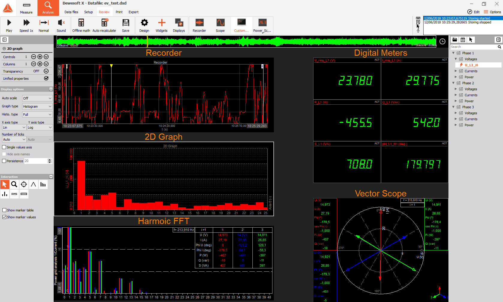
As illustrated in the following images, an unbalanced system can be rectified using the positive, negative and zero symmetrical components. The image below depicts an unsymmetrical system as a screen shot taken from Dewesoft X.


Image 28: Unbalanced system vectorscope in Dewesoft X
This screen was provided by Kurt STRANNER (KNG Netz GmbH)

 The following image depicts a screen-shot showing the three systems (positive, negative and zero) of the symmetrical components in Dewesoft X:

Image 29: Unbalanced system to balanced system transformation in Dewesoft X
This screen was provided by Kurt STRANNER (KNG Netz GmbH) 


Out of the parameters of the symmetrical components (positive-, negative- and zero- sequence) the original system can be rebuilt easily, e.g.:


\[ U_{L1} = U_0 + U_1 + U_2 \]

The following variables are calculated in Dewesoft X and show the components of the zero- and negative-sequence system compared to the positive-sequence system (for the total and the fundamental harmonic).

Table 8: Zero-,positive-, and negative sequence system calculations in the power module 

Extended positive sequence parameters (according to IEC 614000)

The following calculations are based on Annex C of IEC 61400-21.

Based on the measured phase voltages and currents, the fundamental's Fourier coefficients are calculated over one fundamental cycle T as first step.

\[ u_a, cos = \frac{2}{T} \int_{t-T}^t u_a(t) cos (2 \pi f_1 t) dt \]

\[ u_a, sin = \frac{2}{T} \int_{t-T}^t u_a(t) sin (2 \pi f_1 t) dt \]

It is important to mention that the index a stands for the line voltage L1. The coefficients for L2 (ub) and L 3 (uc) as well as the coefficients for the currents (ia, ib, ic) are calculated exactly the same. Furthermore f1 is the frequency of the fundamental. The RMS value of the fundamental line voltage is:

\[U_{a1} = \sqrt {\frac {u^2_{a,cos} +u^2_{a,sin} } {2}} \]

Table 9: Extended positive sequence calculations in the power module  

Extended negative sequence parameters (according to IEC 614000)


Table 10: Extended negative sequence calculations in the power module 


Extended zero sequence parameters (according to IEC 614000)


Table 11: Extended zero sequence calculations in the power module 


Flicker is a term used to describe fluctuations (repetitive variations) of voltage. Flashing light bulbs are indicators of high flicker exposure. Flicker is especially present in grids with a low short-circuit resistance and is caused by the frequent connection and disconnection (e.g. heat pumps, rolling mills, etc.) of loads which affect the voltage. A high level of flicker is perceived as psychologically irritating and can be harmful to humans.Image 30: Flicker impact on humans

 The Dewesoft Power Analyzer can measure all the Flicker parameters according to the IEC 61000-4-15 standard. The Flicker emission calculation is implemented according to the IEC 61400-21 standard and allows for the evaluation of flicker emissions that are fed into the grid by wind power plants and other power generation units.

The flicker-meter architecture is depicted as a block diagram in the next image. It is divided into two parts, simulation of the response to the lamp-eye-brain chain and the on-line statistical analysis of the flicker signal leading to the known parameters. The blocks within the block diagram will be discussed briefly.


Image 31: Flicker-meter architecture 

Block 1

The first block contains a voltage adapting circuit that scales the input mains frequency voltage to an internal reference level. This method permits flicker measurements to be made, independently of the actual input carrier voltage level and may be expressed as a percent ratio.

Block 2

The second block has the function of recovering the voltage fluctuation by squaring the input voltage scaled to the reference level, thus simulating the behavior of a lamp.

Block 3

The third block is composed of a cascade of two filters, which can precede or follow the selective filter circuit. The first low-pass filter eliminates the double mains frequency ripple components of the demodulated output.

The high pass filter can then be used to eliminate any DC voltage component. The second filter is a weighting filter block that simulates the frequency response of the human visual system to sinusoidal voltage fluctuations of a coiled filament gas-filled lamp (60 W/230 V and/or 60 W/120 V).

Block 4

The fourth block consists of a squaring multiplier and a first order low-pass filter. The human flicker perception, with an eye and brain combination, to voltage fluctuations applied to the reference lamp, is simulated by the combined non-linear response of the blocks 2,3 and 4.

Block 5

The last block of the chain performs an on-line analysis of the flicker level, thus allowing direct calculation of significant evaluation parameters.

The following image is an example of a rectangular voltage flicker.

 Image 32: Rectangular voltage flicker 


With Dewesoft X the Short-Term Perceptibility (Pst) and Long-Term Perceptibility (Plt) values can be calculated according to the IEC standard, with a calculation time of 10 minutes and 120 minutes respectively. It is of course also possible to adapt the calculation time to the needs of the user, simply set a calculation overlap and filter.Image 33: Voltage flicker options in the power module
 

Image 34: Flicker measurement screen 


Flicker emission

The flicker emission (also called current flicker) calculates the proportion of the flicker, which is added to the grid by a producer or a consumer. In addition, the internal voltage drop is calculated by the grid impedance of the current flow.

Image 35: Flicker emission options in the power moduleThe voltage drop is added to an idealized voltage source vectorially (U=Usim+R∙I+L∙di/dt). Using the flicker algorithm and the new voltage, the current flicker values are calculated.

Image 36: Schematic illustration of the current flicker calculation Enable "Flicker" and "Flicker emission" and add the grid parameters. The short circuit and the impedance of the grid can then also be added. The phase will be the impedance phase of the grid. The number of different phase angles can also be added (e.g. 30;50;70;85).


The following table expresses the channel names of the different parameters as they are presented in the Dewesoft X software. All the parameters are calculated using the IEC 61000-4-15 Standard's predefined calculation methods.

Table 12: Flicker calculations according to IEC 61000-4-15 


Rapid Voltage Changes are parameters which are added as a supplement to the flicker standard. Rapid Voltage Changes describe all voltage changes that change the voltage for more than 3% at a certain time interval. These voltage changes can afterwards be analyzed with different parameters (depth of voltage change, duration, steady state deviation, etc.).

The Rapid Voltage Changes (RVC) are special calculations in Dewesoft X which allows the calculation of the maximal voltage drop (dmax), the stationary deviation after the voltage drop (dc) and the time where the voltage drops below 3,3% of Un. All values are calculated according to the IEC 61000-4-15. Analysis can be done for example for IEC 61000-3-3 and IEC 61000-3-11. The following image shows the calculated parameters (IEC 61000-4-15 page 35).Image 37: Rapid voltage changes according to the IEC 61000-4-15 standard

Measurements with Dewesoft X

RVCs measurements with Dewesoft X:

Image 38: Rapid voltage change options in the power module

Steady state duration: This defines the duration of the steady state defined in seconds.

Hysteresis: This is the condition for the stationary deviation (du_dc) defined in percentage, see IEC 61000-4-15 page 8.

Example: If a hysteresis of 0,2% and a steady state duration of 1s is defined, the stationary condition is reached if the voltage doesn't deviate more than +- 0,2% for 1 second.


Table 13: Additional flicker calculations according to IEC 61000-4-15

Image 39: Rapid voltage change measurement screen 


DEWESoft has created a special FFT algorithm (software PLL) to determine the periodic time (frequency). The algorithm determines the periodic time of the signal via a special FFT algorithm at a sampling window of multiple periods (typically 10 periods, definable in power module). The calculated frequency is highly accurate (mHz) and works for all applications (motor, inverter, grid, etc.).

How Dewesoft X calculates the power of an AC system

While other power analyses calculate the power in the time domain, in Dewesoft X calculates in the frequency domain. With the predetermined period time, an FFT analysis for voltage and current is done for a definable number of periods (typically 10, with electrical applications) and a definable sampling rate. The FFT yields an amplitude for the voltage, current, and the cos phi for each harmonic. One major benefit of this FFT transformation is that the behavior of amplifiers, current or voltage transducers in amplitude and phase for the whole frequency range (using the Sensor XML) can now be corrected. This way of power analysis has the highest possible accuracy. Another benefit is that harmonic analysis and other power quality analysis can be done completely synchronized to the fundamental frequency.

With the FFT corrected values, the RMS voltages and currents are calculated out of the RMS values of each harmonic.

\[ U_{rms_{total}} = \sqrt {U_0^2 + U_1^2 + U_2^2 + \cdot \cdot \cdot + U_n^2 } \]

\[ I_{rms_{total}} = \sqrt {I_0^2 + I_1^2 + I_2^2 + \cdot \cdot \cdot + I_n^2 } \]

The rectified mean is the average of the rectified signal. In terms of an AC signal, it's the average of the absolute value of voltage or current.

\[ U_{RECT} = \frac {1}{T} \int_{t=0}^T \big| u \big| (t) dt \]

\[ I_{RECT} = \frac {1}{T} \int_{t=0}^T \big| i \big| (t) dt \]

The rectified mean is used e.g. for transformer testing as the rectified mean is proportional to the magnetic flux.

The power values for each harmonic and the total values are calculated with the following formulas:

There are two definitions for reactive power included, because there is up to date no official definition that has been standardized. The formula of Q1_L1 loses sign, while QH_L1 does not. If there is a need to calculate the reactive power form only the harmonics (no fundamental included) the following simple math formula can be used: ‘QH_L1’ – ‘Q_L1_H1’


Power grid

  • fault and transient recording
  • power quality analysis (IEEE 1159, EN50160)

Transformer

  • efficiency analysis (IEC 60076-1)
  • no-load and short circuit testing
  • vibration, noise

Wind, solar and CHP

  • power performance (IEC 61400-12)
  • power quality (IEC 61400-21 / FGW-TR3)
  • active and reactive power (FGW-TR3)
  • behavior at faults (FGW-TR3)

Nuclear power plant

  • turbine and generator
  • testing rod drop
  • castor testing

Turbine and generator

  • modal analysis
  • order tracking
  • balancing
  • rotational vibration
  • efficiency measurement

Smart grid and energy management

  • power system testing
  • load profile
  • demand-side management

Aircraft

  • power system testing
  • fault and transient recording
  • hybrid testing
  • harmonics analysis

Marine

  • power system testing
  • fault and transient recording
  • hybrid testing

Railway

  • power system testing (AC and DC rails)
  • power quality analysis
  • fault and transient recording
  • short-circuit analysis
  • pantograph and current shoe testing

E-mobility

  • electric two-wheeler
  • electric vehicle
  • hybrid vehicle (series and parallel)
  • hydrogen vehicle

Equipment testing

  • fans and pumps testing
  • circuit breaker testing
  • filter analysis
  • harmonics analysis according to IEC 61000-3-2/-12
  • voltage changes according to IEC 61000-3-3/-11
  • CE conformity of electrical devices (harmonics, flicker) and a lot more

To learn more about POWER APPLICATION please download our POWER BROCHURE.

NOTE:  Bandwidth at 1MS/16Bit depends on selected input: HS-LV has 1MHz and HS-HV has 2MHz.